


Let’s begin at the beginning. What do terms like statistical population, statistical comparison, statistical inference mean? What good is munging, coding, booting, regularization etc.
On a scale of 1 to 30 (1 being the lowest and 30, the highest), rate yourself as a data scientist. No matter what you have scored yourself, we hope to have improved that score at least by a little, by the end of this post.
Let’s start with a basic question: What is data science?
[box type=”shadow” align=”” class=”” width=””]The following is an excerpt from the book, Statistics for Data Science written by James D. Miller and published by Packt Publishing.[/box]
The idea of how data science is defined is a matter of opinion.
I personally like the explanation that data science is a progression or, even better, an evolution of thought or steps, as shown in the following figure:
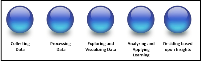
Although a progression or evolution implies a sequential journey, in practice, this is an extremely fluid process; each of the phases may inspire the data scientist to reverse and repeat one or more of the phases until they are satisfied. In other words, all or some phases of the process may be repeated until the data scientist determines that the desired outcome is reached.
Depending on your sources and individual beliefs, you may say the following:
Statistics is data science, and data science is statistics.
Based upon personal experience, research, and various industry experts’ advice, someone delving into the art of data science should take every opportunity to understand and gain experience as well as proficiency with the following list of common data science terms:
- Statistical population
- Probability
- False positives
- Statistical inference
- Regression
- Fitting
- Categorical data
- Classification
- Clustering
- Statistical comparison
- Coding
- Distributions
- Data mining
- Decision trees
- Machine learning
- Munging and wrangling
- Visualization
- D3
- Regularization
- Assessment
- Cross-validation
- Neural networks
- Boosting
- Lift
- Mode
- Outlier
- Predictive modeling
- Big data
- Confidence interval
- Writing
Statistical population
You can perhaps think of a statistical population as a recordset (or a set of records). This set or group of records will be of similar items or events that are of interest to the data scientist for some experiment.
For a data developer, a population of data may be a recordset of all sales transactions for a month, and the interest might be reporting to the senior management of an organization which products are the fastest sellers and at which time of the year.
For a data scientist, a population may be a recordset of all emergency room admissions during a month, and the area of interest might be to determine the statistical demographics for emergency room use.
[box type=”note” align=”” class=”” width=””]Typically, the terms statistical population and statistical model are or can be used interchangeably. Once again, data scientists continue to evolve with their alignment on their use of common terms. [/box]
Another key point concerning statistical populations is that the recordset may be a group of (actually) existing objects or a hypothetical group of objects. Using the preceding example, you might draw a comparison of actual objects as those actual sales transactions recorded for the month while the hypothetical objects as sales transactions are expected, forecast, or presumed (based upon observations or experienced assumptions or other logic) to occur during a month.
Finally, through the use of statistical inference, the data scientist can select a portion or subset of the recordset (or population) with the intention that it will represent the total population for a particular area of interest. This subset is known as a statistical sample.
If a sample of a population is chosen accurately, characteristics of the entire population (that the sample is drawn from) can be estimated from the corresponding characteristics of the sample.
Probability
Probability is concerned with the laws governing random events. -www.britannica.com
When thinking of probability, you think of possible upcoming events and the likelihood of them actually occurring. This compares to a statistical thought process that involves analyzing the frequency of past events in an attempt to explain or make sense of the observations. In addition, the data scientist will associate various individual events, studying the relationship of these events. How these different events relate to each other governs the methods and rules that will need to be followed when we’re studying their probabilities.
[box type=”note” align=”” class=”” width=””]A probability distribution is a table that is used to show the probabilities of various outcomes in a sample population or recordset. [/box]
False positives
The idea of false positives is a very important statistical (data science) concept. A false positive is a mistake or an errored result. That is, it is a scenario where the results of a process or experiment indicate a fulfilled or true condition when, in fact, the condition is not true (not fulfilled). This situation is also referred to by some data scientists as a false alarm and is most easily understood by considering the idea of a recordset or statistical population (which we discussed earlier in this section) that is determined not only by the accuracy of the processing but by the characteristics of the sampled population. In other words, the data scientist has made errors during the statistical process, or the recordset is a population that does not have an appropriate sample (or characteristics) for what is being investigated.
Statistical inference
What developer at some point in his or her career, had to create a sample or test data? For example, I’ve often created a simple script to generate a random number (based upon the number of possible options or choices) and then used that number as the selected option (in my test recordset). This might work well for data development, but with statistics and data science, this is not sufficient.
To create sample data (or a sample population), the data scientist will use a process called statistical inference, which is the process of deducing options of an underlying distribution through analysis of the data you have or are trying to generate for. The process is sometimes called inferential statistical analysis and includes testing various hypotheses and deriving estimates.
When the data scientist determines that a recordset (or population) should be larger than it actually is, it is assumed that the recordset is a sample from a larger population, and the data scientist will then utilize statistical inference to make up the difference.
[box type=”note” align=”” class=”” width=””]The data or recordset in use is referred to by the data scientist as the observed data. Inferential statistics can be contrasted with descriptive statistics, which is only concerned with the properties of the observed data and does not assume that the recordset came from a larger population. [/box]
Regression
Regression is a process or method (selected by the data scientist as the best fit technique for the experiment at hand) used for determining the relationships among variables. If you’re a programmer, you have a certain understanding of what a variable is, but in statistics, we use the term differently. Variables are determined to be either dependent or independent.
An independent variable (also known as a predictor) is the one that is manipulated by the data scientist in an effort to determine its relationship with a dependent variable. A dependent variable is a variable that the data scientist is measuring.
[box type=”note” align=”” class=”” width=””]It is not uncommon to have more than one independent variable in a data science progression or experiment. [/box]
More precisely, regression is the process that helps the data scientist comprehend how the typical value of the dependent variable (or criterion variable) changes when any one or more of the independent variables is varied while the other independent variables are held fixed.
Fitting
Fitting is the process of measuring how well a statistical model or process describes a data scientist’s observations pertaining to a recordset or experiment. These measures will attempt to point out the discrepancy between observed values and probable values. The probable values of a model or process are known as a distribution or a probability distribution.
Therefore, a probability distribution fitting (or distribution fitting) is when the data scientist fits a probability distribution to a series of data concerning the repeated measurement of a variable phenomenon.
The object of a data scientist performing a distribution fitting is to predict the probability or to forecast the frequency of, the occurrence of the phenomenon at a certain interval.
[box type=”note” align=”” class=”” width=””]One of the most common uses of fitting is to test whether two samples are drawn from identical distributions.[/box]
There are numerous probability distributions a data scientist can select from. Some will fit better to the observed frequency of the data than others will. The distribution giving a close fit is supposed to lead to good predictions; therefore, the data scientist needs to select a distribution that suits the data well.
Categorical data
Earlier, we explained how variables in your data can be either independent or dependent. Another type of variable definition is a categorical variable. This type of variable is one that can take on one of a limited, and typically fixed, number of possible values, thus assigning each individual to a particular category.
Often, the collected data’s meaning is unclear. Categorical data is a method that a data scientist can use to put meaning to the data.
For example, if a numeric variable is collected (let’s say the values found are 4, 10, and 12), the meaning of the variable becomes clear if the values are categorized. Let’s suppose that based upon an analysis of how the data was collected, we can group (or categorize) the data by indicating that this data describes university students, and there is the following number of players:
- 4 tennis players
- 10 soccer players
- 12 football players
Now, because we grouped the data into categories, the meaning becomes clear.
Some other examples of categorized data might be individual pet preferences (grouped by the type of pet), or vehicle ownership (grouped by the style of a car owned), and so on.
So, categorical data, as the name suggests, is data grouped into some sort of category or multiple categories. Some data scientists refer to categories as sub-populations of data.
[box type=”note” align=”” class=”” width=””]Categorical data can also be data that is collected as a yes or no answer. For example, hospital admittance data may indicate that patients either smoke or do not smoke. [/box]
Classification
Statistical classification of data is the process of identifying which category (discussed in the previous section) a data point, observation, or variable should be grouped into. The data science process that carries out a classification process is known as a classifier.
Read this post: Classification using Convolutional Neural Networks
[box type=”note” align=”” class=”” width=””]Determining whether a book is fiction or non-fiction is a simple example classification. An analysis of data about restaurants might lead to the classification of them among several genres. [/box]
Clustering
Clustering is the process of dividing up the data occurrences into groups or homogeneous subsets of the dataset, not a predetermined set of groups as in classification (described in the preceding section) but groups identified by the execution of the data science process based upon similarities that it found among the occurrences.
Objects in the same group (a group is also referred to as a cluster) are found to be more analogous (in some sense or another) to each other than to those objects found in other groups (or found in other clusters). The process of clustering is found to be very common in exploratory data mining and is also a common technique for statistical data analysis.
Statistical comparison
Simply put, when you hear the term statistical comparison, one is usually referring to the act of a data scientist performing a process of analysis to view the similarities or variances of two or more groups or populations (or recordsets).
As a data developer, one might be familiar with various utilities such as FC Compare, UltraCompare, or WinDiff, which aim to provide the developer with a line-by-line comparison of the contents of two or more (even binary) files.
In statistics (data science), this process of comparing is a statistical technique to compare populations or recordsets. In this method, a data scientist will conduct what is called an Analysis of Variance (ANOVA), compare categorical variables (within the recordsets), and so on.
[box type=”note” align=”” class=”” width=””]ANOVA is an assortment of statistical methods that are used to analyze the differences among group means and their associated procedures (such as variations among and between groups, populations, or recordsets). This method eventually evolved into the Six Sigma dataset comparisons. [/box]
Coding
Coding or statistical coding is again a process that a data scientist will use to prepare data for analysis. In this process, both quantitative data values (such as income or years of education) and qualitative data (such as race or gender) are categorized or coded in a consistent way.
Coding is performed by a data scientist for various reasons such as follows:
- More effective for running statistical models
- Computers understand the variables
- Accountability–so the data scientist can run models blind, or without knowing what variables stand for, to reduce programming/author bias
[box type=”shadow” align=”” class=”” width=””]You can imagine the process of coding as the means to transform data into a form required for a system or application. [/box]
Distributions
The distribution of a statistical recordset (or of a population) is a visualization showing all the possible values (or sometimes referred to as intervals) of the data and how often they occur. When a distribution of categorical data (which we defined earlier in this chapter) is created by a data scientist, it attempts to show the number or percentage of individuals in each group or category.
Linking an earlier defined term with this one, a probability distribution, stated in simple terms, can be thought of as a visualization showing the probability of occurrence of different possible outcomes in an experiment.
Data mining
With data mining, one is usually more absorbed in the data relationships (or the potential relationships between points of data, sometimes referred to as variables) and cognitive analysis.
To further define this term, we can say that data mining is sometimes more simply referred to as knowledge discovery or even just discovery, based upon processing through or analyzing data from new or different viewpoints and summarizing it into valuable insights that can be used to increase revenue, cuts costs, or both.
Using software dedicated to data mining is just one of several analytical approaches to data mining. Although there are tools dedicated to this purpose (such as IBM Cognos BI and Planning Analytics, Tableau, SAS, and so on.), data mining is all about the analysis process finding correlations or patterns among dozens of fields in the data and that can be effectively accomplished using tools such as MS Excel or any number of open source technologies.
[box type=”note” align=”” class=”” width=””]A common technique to data mining is through the creation of custom scripts using tools such as R or Python. In this way, the data scientist has the ability to customize the logic and processing to their exact project needs. [/box]
Decision trees
A statistical decision tree uses a diagram that looks like a tree. This structure attempts to represent optional decision paths and a predicted outcome for each path selected. A data scientist will use a decision tree to support, track, and model decision making and their possible consequences, including chance event outcomes, resource costs, and utility. It is a common way to display the logic of a data science process.
Machine learning
Machine learning is one of the most intriguing and exciting areas of data science. It conjures all forms of images around artificial intelligence which includes Neural Networks, Support Vector Machines (SVMs), and so on.
Fundamentally, we can describe the term machine learning as a method of training a computer to make or improve predictions or behaviors based on data or, specifically, relationships within that data. Continuing, machine learning is a process by which predictions are made based upon recognized patterns identified within data, and additionally, it is the ability to continuously learn from the data’s patterns, therefore continuingly making better predictions.
It is not uncommon for someone to mistake the process of machine learning for data mining, but data mining focuses more on exploratory data analysis and is known as unsupervised learning.
Machine learning can be used to learn and establish baseline behavioral profiles for various entities and then to find meaningful anomalies.
Here is the exciting part: the process of machine learning (using data relationships to make predictions) is known as predictive analytics.
Predictive analytics allow the data scientists to produce reliable, repeatable decisions and results and uncover hidden insights through learning from historical relationships and trends in the data.
Munging and wrangling
The terms munging and wrangling are buzzwords or jargon meant to describe one’s efforts to affect the format of data, recordset, or file in some way in an effort to prepare the data for continued or otherwise processing and/or evaluations.
With data development, you are most likely familiar with the idea of Extract, Transform, and Load (ETL). In somewhat the same way, a data developer may mung or wrangle data during the transformation steps within an ETL process.
Common munging and wrangling may include removing punctuation or HTML tags, data parsing, filtering, all sorts of transforming, mapping, and tying together systems and interfaces that were not specifically designed to interoperate. Munging can also describe the processing or filtering of raw data into another form, allowing for more convenient consumption of the data elsewhere.
Munging and wrangling might be performed multiple times within a data science process and/or at different steps in the evolving process. Sometimes, data scientists use munging to include various data visualization, data aggregation, training a statistical model, as well as much other potential work. To this point, munging and wrangling may follow a flow beginning with extracting the data in a raw form, performing the munging using various logic, and lastly, placing the resulting content into a structure for use.
Although there are many valid options for munging and wrangling data, preprocessing and manipulation, a tool that is popular with many data scientists today is a product named Trifecta, which claims that it is the number one (data) wrangling solution in many industries.
[box type=”note” align=”” class=”” width=””]Trifecta can be downloaded for your personal evaluation from https://www.trifacta.com/. Check it out! [/box]
Visualization
The main point (although there are other goals and objectives) when leveraging a data visualization technique is to make something complex appear simple. You can think of visualization as any technique for creating a graphic (or similar) to communicate a message.
Other motives for using data visualization include the following:
- To explain the data or put the data in context (which is to highlight demographic statistics)
- To solve a specific problem (for example, identifying problem areas within a particular business model)
- To explore the data to reach a better understanding or add clarity (such as what periods of time do this data span?)
- To highlight or illustrate otherwise invisible data (such as isolating outliers residing in the data)
- To predict, such as potential sales volumes (perhaps based upon seasonality sales statistics)
- And others
Statistical visualization is used in almost every step in the data science process, within the obvious steps such as exploring and visualizing, analyzing and learning, but can also be leveraged during collecting, processing, and the end game of using the identified insights.
D3
D3 or D3.js, is essentially an open source JavaScript library designed with the intention of visualizing data using today’s web standards. D3 helps put life into your data, utilizing Scalable Vector Graphics (SVG), Canvas, and standard HTML.
D3 combines powerful visualization and interaction techniques with a data-driven approach to DOM manipulation, providing data scientists with the full capabilities of modern browsers and the freedom to design the right visual interface that best depicts the objective or assumption.
In contrast to many other libraries, D3.js allows inordinate control over the visualization of data. D3 is embedded within an HTML webpage and uses pre-built JavaScript functions to select elements, create SVG objects, style them, or add transitions, dynamic effects, and so on.
Regularization
Regularization is one possible approach that a data scientist may use for improving the results generated from a statistical model or data science process, such as when addressing a case of overfitting in statistics and data science.
[box type=”note” align=”” class=”” width=””]We defined fitting earlier (fitting describes how well a statistical model or process describes a data scientist’s observations). Overfitting is a scenario where a statistical model or process seems to fit too well or appears to be too close to the actual data.[/box]
Overfitting usually occurs with an overly simple model. This means that you may have only two variables and are drawing conclusions based on the two. For example, using our previously mentioned example of daffodil sales, one might generate a model with temperature as an independent variable and sales as a dependent one. You may see the model fail since it is not as simple as concluding that warmer temperatures will always generate more sales.
In this example, there is a tendency to add more data to the process or model in hopes of achieving a better result. The idea sounds reasonable. For example, you have information such as average rainfall, pollen count, fertilizer sales, and so on; could these data points be added as explanatory variables?
[box type=”note” align=”” class=”” width=””]An explanatory variable is a type of independent variable with a subtle difference. When a variable is independent, it is not affected at all by any other variables. When a variable isn’t independent for certain, it’s an explanatory variable. [/box]
Continuing to add more and more data to your model will have an effect but will probably cause overfitting, resulting in poor predictions since it will closely resemble the data, which is mostly just background noise.
To overcome this situation, a data scientist can use regularization, introducing a tuning parameter (additional factors such as a data points mean value or a minimum or maximum limitation, which gives you the ability to change the complexity or smoothness of your model) into the data science process to solve an ill-posed problem or to prevent overfitting.
Assessment
When a data scientist evaluates a model or data science process for performance, this is referred to as assessment. Performance can be defined in several ways, including the model’s growth of learning or the model’s ability to improve (with) learning (to obtain a better score) with additional experience (for example, more rounds of training with additional samples of data) or accuracy of its results.
One popular method of assessing a model or processes performance is called bootstrap sampling. This method examines performance on certain subsets of data, repeatedly generating results that can be used to calculate an estimate of accuracy (performance).
The bootstrap sampling method takes a random sample of data, splits it into three files–a training file, a testing file, and a validation file. The model or process logic is developed based on the data in the training file and then evaluated (or tested) using the testing file. This tune and then test process is repeated until the data scientist is comfortable with the results of the tests. At that point, the model or process is again tested, this time using the validation file, and the results should provide a true indication of how it will perform.
[box type=”note” align=”” class=”” width=””]You can imagine using the bootstrap sampling method to develop program logic by analyzing test data to determine logic flows and then running (or testing) your logic against the test data file. Once you are satisfied that your logic handles all of the conditions and exceptions found in your testing data, you can run a final test on a new, never-before-seen data file for a final validation test. [/box]
Cross-validation
Cross-validation is a method for assessing a data science process performance. Mainly used with predictive modeling to estimate how accurately a model might perform in practice, one might see cross-validation used to check how a model will potentially generalize, in other words, how the model can apply what it infers from samples to an entire population (or recordset).
With cross-validation, you identify a (known) dataset as your validation dataset on which training is run along with a dataset of unknown data (or first seen data) against which the model will be tested (this is known as your testing dataset). The objective is to ensure that problems such as overfitting (allowing non-inclusive information to influence results) are controlled and also provide an insight into how the model will generalize a real problem or on a real data file.
The cross-validation process will consist of separating data into samples of similar subsets, performing the analysis on one subset (called the training set) and validating the analysis on the other subset (called the validation set or testing set). To reduce variability, multiple iterations (also called folds or rounds) of cross-validation are performed using different partitions, and the validation results are averaged over the rounds. Typically, a data scientist will use a models stability to determine the actual number of rounds of cross-validation that should be performed.
Neural networks
Neural networks are also called artificial neural networks (ANNs), and the objective is to solve problems in the same way that the human brain would.
Google will provide the following explanation of ANN as stated in Neural Network Primer: Part I, by Maureen Caudill, AI Expert, Feb. 1989:
[box type=”note” align=”” class=”” width=””]A computing system made up of several simple, highly interconnected processing elements, which process information by their dynamic state response to external inputs. [/box]
To oversimplify the idea of neural networks, recall the concept of software encapsulation, and consider a computer program with an input layer, a processing layer, and an output layer. With this thought in mind, understand that neural networks are also organized in a network of these layers, usually with more than a single processing layer.
Patterns are presented to the network by way of the input layer, which then communicates to one (or more) of the processing layers (where the actual processing is done). The processing layers then link to an output layer where the result is presented.
Most neural networks will also contain some form of learning rule that modifies the weights of the connections (in other words, the network learns which processing nodes perform better and gives them a heavier weight) per the input patterns that it is presented with. In this way (in a sense), neural networks learn by example as a child learns to recognize a cat from being exposed to examples of cats.
Boosting
In a manner of speaking, boosting is a process generally accepted in data science for improving the accuracy of a weak learning data science process.
[box type=”note” align=”” class=”” width=””]Data science processes defined as weak learners are those that produce results that are only slightly better than if you would randomly guess the outcome. Weak learners are basically thresholds or a 1-level decision tree. [/box]
Specifically, boosting is aimed at reducing bias and variance in supervised learning.
What do we mean by bias and variance? Before going on further about boosting, let’s take note of what we mean by bias and variance.
Data scientists describe bias as a level of favoritism that is present in the data collection process, resulting in uneven, disingenuous results and can occur in a variety of different ways. A sampling method is called biased if it systematically favors some outcomes over others.
A variance may be defined (by a data scientist) simply as the distance from a variable mean (or how far from the average a result is).
The boosting method can be described as a data scientist repeatedly running through a data science process (that has been identified as a weak learning process), with each iteration running on different and random examples of data sampled from the original population recordset. All the results (or classifiers or residue) produced by each run are then combined into a single merged result (that is a gradient).
This concept of using a random subset of the original recordset for each iteration originates from bootstrap sampling in bagging and has a similar variance-reducing effect on the combined model.
In addition, some data scientists consider boosting a means to convert weak learners into strong ones; in fact, to some, the process of boosting simply means turning a weak learner into a strong learner.
Lift
In data science, the term lift compares the frequency of an observed pattern within a recordset or population with how frequently you might expect to see that same pattern occur within the data by chance or randomly.
If the lift is very low, then typically, a data scientist will expect that there is a very good probability that the pattern identified is occurring just by chance. The larger the lift, the more likely it is that the pattern is real.
Mode
In statistics and data science, when a data scientist uses the term mode, he or she refers to the value that occurs most often within a sample of data. Mode is not calculated but is determined manually or through processing of the data.
Outlier
Outliers can be defined as follows:
- A data point that is way out of keeping with the others
- That piece of data that doesn’t fit
- Either a very high value or a very low value
- Unusual observations within the data
- An observation point that is distant from all others
Predictive modeling
The development of statistical models and/or data science processes to predict future events is called predictive modeling.
Big Data
Again, we have some variation of the definition of big data. A large assemblage of data, data sets that are so large or complex that traditional data processing applications are inadequate, and data about every aspect of our lives have all been used to define or refer to big data. In 2001, then Gartner analyst Doug Laney introduced the 3V’s concept.
The 3V’s, as per Laney, are volume, variety, and velocity. The V’s make up the dimensionality of big data: volume (or the measurable amount of data), variety (meaning the number of types of data), and velocity (referring to the speed of processing or dealing with that data).
Confidence interval
The confidence interval is a range of values that a data scientist will specify around an estimate to indicate their margin of error, combined with a probability that a value will fall in that range. In other words, confidence intervals are good estimates of the unknown population parameter.
Writing
Although visualizations grab much more of the limelight when it comes to presenting the output or results of a data science process or predictive model, writing skills are still not only an important part of how a data scientist communicates but still considered an essential skill for all data scientists to be successful.
Did we miss any of your favorite terms? Now that you are at the end of this post, we ask you again: On a scale of 1 to 30 (1 being the lowest and 30, the highest), how do you rate yourself as a data scientist?


