


In today’s tutorial, we will efficiently train our first predictive model, we will use Cross-validation in R as the basis of our modeling process. We will build the corresponding confusion matrix. Most of the functionality comes from the excellent caret package. You can find more information on the vast features of caret package that we will not explore in this tutorial.
Before moving to the training tutorial, lets understand what a confusion matrix is. A confusion matrix is a summary of prediction results on a classification problem. The number of correct and incorrect predictions are summarized with count values and broken down by each class. This is the key to the confusion matrix. The confusion matrix shows the ways in which your classification model is confused when it makes predictions. It gives you insight not only into the errors being made by your classifier but more importantly the types of errors that are being made.
Training our first predictive model
Following best practices, we will use Cross Validation (CV) as the basis of our modeling process. Using CV we can create estimates of how well our model will do with unseen data. CV is powerful, but the downside is that it requires more processing and therefore more time. If you can take the computational complexity, you should definitely take advantage of it in your projects.
Going into the mathematics behind CV is outside of the scope of this tutorial. If interested, you can find out more information on cross validation on Wikipedia . The basic idea is that the training data will be split into various parts, and each of these parts will be taken out of the rest of the training data one at a time, keeping all remaining parts together. The parts that are kept together will be used to train the model, while the part that was taken out will be used for testing, and this will be repeated by rotating the parts such that every part is taken out once. This allows you to test the training procedure more thoroughly, before doing the final testing with the testing data.
We use the trainControl() function to set our repeated CV mechanism with five splits and two repeats. This object will be passed to our predictive models, created with the caret package, to automatically apply this control mechanism within them:
cv.control <- trainControl(method = "repeatedcv", number = 5, repeats = 2)Our predictive models pick for this example are Random Forests (RF). We will very briefly explain what RF are, but the interested reader is encouraged to look into James, Witten, Hastie, and Tibshirani’s excellent “Statistical Learning” (Springer, 2013). RF are a non-linear model used to generate predictions. A tree is a structure that provides a clear path from inputs to specific outputs through a branching model. In predictive modeling they are used to find limited input-space areas that perform well when providing predictions. RF create many such trees and use a mechanism to aggregate the predictions provided by this trees into a single prediction. They are a very powerful and popular Machine Learning model.
Let’s have a look at the random forests example:
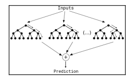
Random forests aggregate trees
To train our model, we use the train() function passing a formula that signals R to use MULT_PURCHASES as the dependent variable and everything else (~ .) as the independent variables, which are the token frequencies. It also specifies the data, the method (“rf” stands for random forests), the control mechanism we just created, and the number of tuning scenarios to use:
model.1 <- train(

MULT_PURCHASES ~ .,

data = train.dfm.df,

method = "rf",

trControl = cv.control,

tuneLength = 5

)
Improving speed with parallelization
If you actually executed the previous code in your computer before reading this, you may have found that it took a long time to finish (8.41 minutes in our case). As we mentioned earlier, text analysis suffers from very high dimensional structures which take a long time to process. Furthermore, using CV runs will take a long time to run. To cut down on the total execution time, use the doParallel package to allow for multi-core computers to do the training in parallel and substantially cut down on time.
We proceed to create the train_model() function, which takes the data and the control mechanism as parameters. It then makes a cluster object with the makeCluster() function with a number of available cores (processors) equal to the number of cores in the computer, detected with the detectCores() function. Note that if you’re planning on using your computer to do other tasks while you train your models, you should leave one or two cores free to avoid choking your system (you can then use makeCluster(detectCores() –2) to accomplish this). After that, we start our time measuring mechanism, train our model, print the total time, stop the cluster, and return the resulting model.
train_model <- function(data, cv.control) {

cluster <- makeCluster(detectCores())

registerDoParallel(cluster)

start.time <- Sys.time()

model <- train(

MULT_PURCHASES ~ .,

data = data,

method = "rf",

trControl = cv.control,

tuneLength = 5

)

print(Sys.time() - start.time)

stopCluster(cluster)

return(model)

}
Now we can retrain the same model much faster. The time reduction will depend on your computer’s available resources. In the case of an 8-core system with 32 GB of memory available, the total time was 3.34 minutes instead of the previous 8.41 minutes, which implies that with parallelization, it only took 39% of the original time. Not bad right? Let’s have look at how the model is trained:
model.1 <- train_model(train.dfm.df, cv.control)Computing predictive accuracy and confusion matrices
Now that we have our trained model, we can see its results and ask it to compute some predictive accuracy metrics. We start by simply printing the object we get back from the train() function. As can be seen, we have some useful metadata, but what we are concerned with right now is the predictive accuracy, shown in the Accuracy column. From the five values we told the function to use as testing scenarios, the best model was reached when we used 356 out of the 2,007 available features (tokens). In that case, our predictive accuracy was 65.36%.
If we take into account the fact that the proportions in our data were around 63% of cases with multiple purchases, we have made an improvement. This can be seen by the fact that if we just guessed the class with the most observations (MULT_PURCHASES being true) for all the observations, we would only have a 63% accuracy, but using our model we were able to improve toward 65%. This is a 3% improvement.
Keep in mind that this is a randomized process, and the results will be different every time you train these models. That’s why we want a repeated CV as well as various testing scenarios to make sure that our results are robust:
model.1
#> Random Forest
#>
#> 212 samples
#> 2007 predictors
#> 2 classes: 'FALSE', 'TRUE'
#>
#> No pre-processing
#> Resampling: Cross-Validated (5 fold, repeated 2 times)
#> Summary of sample sizes: 170, 169, 170, 169, 170, 169, ...
#> Resampling results across tuning parameters:
#>
#> mtry Accuracy Kappa
#> 2 0.6368771 0.00000000
#> 11 0.6439092 0.03436849
#> 63 0.6462901 0.07827322
#> 356 0.6536545 0.16160573
#> 2006 0.6512735 0.16892126
#>
#> Accuracy was used to select the optimal model using the largest value.
#> The final value used for the model was mtry = 356.
To create a confusion matrix, we can use the confusionMatrix() function and send it the model’s predictions first and the real values second. This will not only create the confusion matrix for us, but also compute some useful metrics such as sensitivity and specificity. We won’t go deep into what these metrics mean or how to interpret them since that’s outside the scope of this tutorial, but we highly encourage the reader to study them using the resources cited in this tutorial:
confusionMatrix(model.1$finalModel$predicted, train$MULT_PURCHASES)
#> Confusion Matrix and Statistics
#>
#> Reference
#> Prediction FALSE TRUE
#> FALSE 18 19
#> TRUE 59 116
#>
#> Accuracy : 0.6321
#> 95% CI : (0.5633, 0.6971)
#> No Information Rate : 0.6368
#> P-Value [Acc > NIR] : 0.5872
#>
#> Kappa : 0.1047
#> Mcnemar's Test P-Value : 1.006e-05
#>
#> Sensitivity : 0.23377
#> Specificity : 0.85926
#> Pos Pred Value : 0.48649
#> Neg Pred Value : 0.66286
#> Prevalence : 0.36321
#> Detection Rate : 0.08491
#> Detection Prevalence : 0.17453
#> Balanced Accuracy : 0.54651
#>
#> 'Positive' Class : FALSE
You read an excerpt from R Programming By Example authored by Omar Trejo Navarro. This book gets you familiar with R’s fundamentals and its advanced features to get you hands-on experience with R’s cutting edge tools for software development.

Read Next
Getting Started with Predictive Analytics
Here’s how you can handle the bias variance trade-off in your ML models


