


In this blog post, we begin with a simple classification task that the reader can readily relate to. The task is a binary classification of 25000 images of cats and dogs, divided into 20000 training, 2500 validation, and 2500 testing images. It seems reasonable to use the most promising model for object recognition, which is convolutional neural network (CNN). As a result, we use CNN as the baseline for the experiments, and along with this post, we will try to improve its performance using different techniques. So, in the next sections, we will first introduce CNN and its architecture and then we will explore three techniques to boost the performance and speed. These three techniques are using Parametric ReLU and a method of Batch Normalization. In this post, we will show the experimental results as we go through each technique. The complete code for CNN is available online in the author’s GitHub repository.
Convolutional Neural Networks
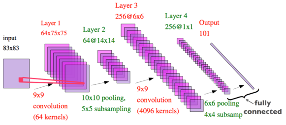
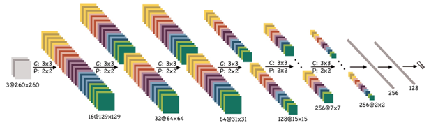
Convolutional neural networks can be seen as feedforward neural networks that multiple copies of the same neuron are applied to in different places. It means applying the same function to different patches of an image. Doing this means that we are explicitly imposing our knowledge about data (images) into the model structure. That’s because we already know that natural image data is translation invariant, meaning that probability distribution of pixels are the same across all images. This structure, which is followed by a non-linearity and a pooling and subsampling layer, makes CNN’s powerful models, especially, when dealing with images. Here’s a graphical illustration of CNN from Prof. Hugo Larochelle’s course of Neural Networks, which is originally from Prof. YannLecun’s paper on ConvNets.
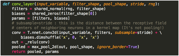
Implementation of a CNN in a GPU-based language of Theano is so straightforward as well. So, we can create a layer like this:
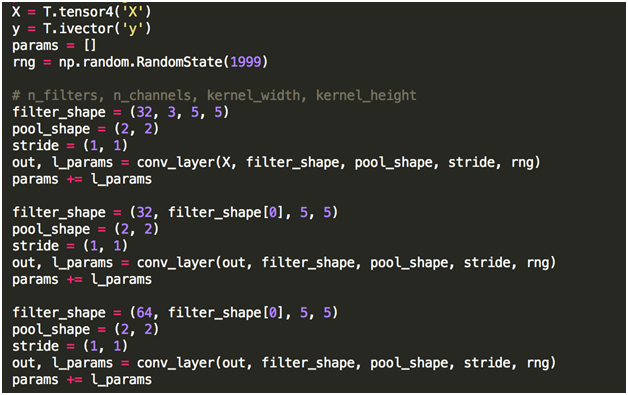
And then we can stack them on top of each other like this:
CNN Experiments
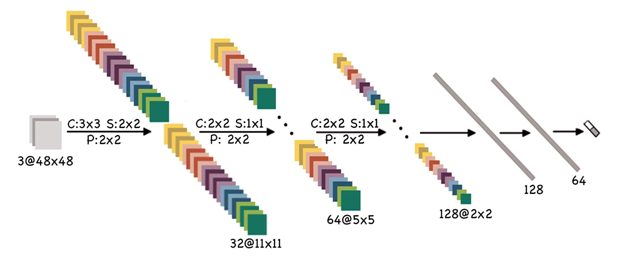
Armed with CNN, we attacked the task using two baseline models. A relatively big, and a relatively small model. In the figures below, you can see the number for layer, filter size, pooling size, stride, and a number of fully connected layers. We trained both networks with a learning rate of 0.01, and a momentum of 0.9 on a GTX580 GPU. We also used early stopping.
The small model can be trained in two hours and results in 81 percent accuracy on validation sets.
The big model can be trained in 24 hours and results in 92 percent accuracy on validation sets.
Parametric ReLU
Parametric ReLU (aka Leaky ReLU) is an extension to Rectified Linear Unitthat allows the neuron to learn the slope of activation function in the negative region. Unlike the actual paper of Parametric ReLU by Microsoft Research, I used a different parameterizationthat forces the slope to be between 0 and 1. As shown in the figure below, when alpha is 0, the activation function is just linear. On the other hand, if alpha is 1, then the activation function is exactly the ReLU. Interestingly, although the number of trainable parameters is increased using Parametric ReLU, it improves the model both in terms of accuracy and in terms of convergence speed. Using Parametric ReLU makes the training time 3/4 and increases the accuracy around 1 percent.
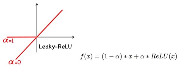
In Parametric ReLU,to make sure that alpha remains between 0 and 1, we will set alpha = Sigmoid(beta) and optimize beta instead. In our experiments, we will set the initial value of alpha to 0.5. After training, all alphas were between 0.5 and 0.8. That means that the model enjoys having a small gradient in the negative region.
“Basically, even a small slope in negative region of activation function can help training a lot. Besides, it’s important to let the model decide how much nonlinearity it needs.”
Batch Normalization
Batch Normalization simply means normalizing preactivations for each batch to have zero mean and unit variance. Based on a recent paper by Google, this normalization reduces a problem called Internal Covariance Shift and consequently makes the learning much faster. The equations are as follows:
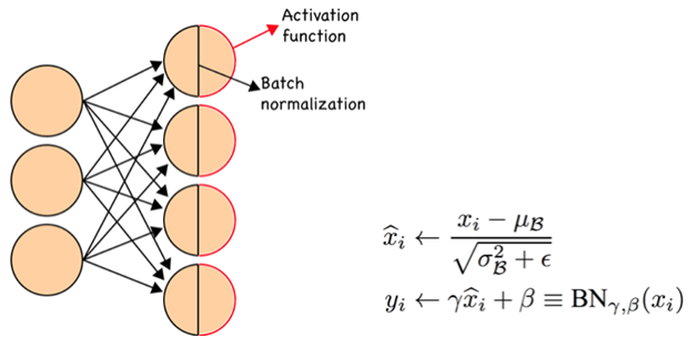
Personally, during this post, I found this as one of the most interesting and simplest techniques I’ve ever used. A very important point to keep in mind is to feed the whole validation set as a single batch at testing time to have a more accurate (less biased) estimation of mean and variance.
“Batch Normalization, which means normalizing pre-activations for each batch to have zero mean and unit variance, can boost the results both in terms of accuracy and in terms of convergence speed.”
Conclusion
All in all, we will conclude this post with two finalized models. One of them can be trained in 10 epochs or, equivalently, 15 minutes, and can achieve 80 percent accuracy. The other model is a relatively large model. In this model, we did not use LDNN, but the two other techniques are used, and we achieved 94.5 percent accuracy.
About the Author
Mohammad Pezeshki is a PhD student in the MILA lab at University of Montreal. He obtained his bachelor’s in computer engineering from Amirkabir University of Technology (Tehran Polytechnic) in July 2014. He then obtained his Master’s in June 2016. His research interests lie in the fields of Artificial Intelligence, Machine Learning, Probabilistic Models and, specifically,Deep Learning.