Implementing Data Modeling techniques in Qlik Sense [Tutorial]

Data modeling is a conceptual process, representing the associations between the data in a manner in which it caters to specific business requirements. In this process, the various data tables are linked as per the business rules to achieve business needs.

In this article, we will look at the basic concept of data modeling, its various types, and learn which technique is best suited for Qlik Sense dashboards. We will also learn about the methods for linking data with each other using joins and concatenation.

Technical requirements

For this article, we will use the app created earlier in the book, as a starting point with a loaded data model. You can find it in the book’s GitHub repository. You can also download the initial and final version of the application from the repository.

After downloading the initial version of the application, perform the following steps:

• If you are using Qlik Sense Desktop, place the app in the Qlik\Sense\Apps folder under your Documents personal folder
• If you are using Qlik Sense Cloud, upload the app to your personal workspace

Advantages of data modeling

Data modeling helps business in many ways. Let’s look at some of the advantages of data modeling:

• High-speed retrieval: Data modeling helps to get the required information much faster than expected. This is because the data is interlinked between the different tables using the relationship.
• Provides ease of accessing data: Data modeling eases the process of giving the right access to the data to the end-users. With the simple data query language, you can get the required data easily.
• Helps in handling multiple relations: Various datasets have various kinds of relationship between the other data. For example, there could be one-to-one, or one-to-many, or many-to-many relationships. Data modeling helps in handling this kind of relationship easily.
• Stability: Data modeling provides stability to the system.

Data modeling techniques

There are various techniques in which data models can be built, each technique has its own advantages and disadvantages. The following are two widely-used data modeling techniques.

Entity-relationship modeling

The entity-relationship modeling (ER modeling) technique uses the entity and relationships to create a logical data model.  This technique is best suited for the Online Transaction Processing (OLTP) systems. An entity in this model refers to anything or object in the real world that has distinguishable characteristics. While a relationship in this model is the relationship between the two or more entities.

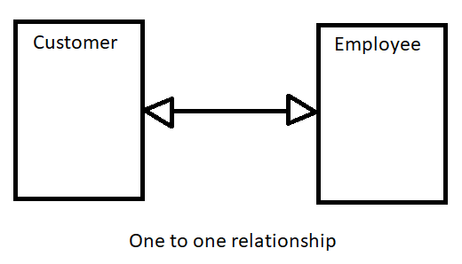
There are three basic types of relationship that can exist:

• One-to-one: This relation means each value from one entity has a single relation with a value from the other entity. For example, one customer is handled by one sales representative:

• One-to-many: This relation means each value from one entity has multiple relations with values from other entities. For example, one sales representative handles multiple customers:

• Many-to-many: This relation means all values from both entities have multiple relations with each other. For example, one book can have many authors and each author can have multiple books:

Dimensional modeling

The dimensional modeling technique uses facts and dimensions to build the data model. This modeling technique was developed by Ralf Kimball. Unlike ER modeling, which uses normalization to build the model, this technique uses the denormalization of data to build the model.

Facts, in this context, are tables that store the most granular transactional details. They mainly store the performance measurement metrics, which are the outcome of the business process. Fact tables are huge in size, because they store the transactional records. For example, let’s say that sales data is captured at a retail store. The fact table for such data would look like the following:

A fact table has the following characteristics:

• It contains the measures, which are mostly numeric in nature
• It stores the foreign key, which refers to the dimension tables
• It stores large numbers of records
• Mostly, it does not contain descriptive data

The dimension table stores the descriptive data, describing the who, what, which, when, how, where, and why associated with the transaction. It has the maximum number of columns, but the records are generally fewer than fact tables. Dimension tables are also referred to as companions of the fact table. They store textual, and sometimes numerical, values. For example, a PIN code is numeric in nature, but they are not the measures and thus they get stored in the dimension table.

In the previous sales example that we discussed, the customer, product, time, and salesperson are the dimension tables. The following diagram shows a sample dimension table:

The following are the characteristics of the dimension table:

• It stores descriptive data, which describes the attributes of the transaction
• It contains many columns and fewer records compared to the fact table
• It also contains numeric data, which is descriptive in nature

There are two types of dimensional modeling techniques that are widely used:

• Star schema: This schema model has one fact table that is linked with multiple dimension tables. The name star is given because once the model is ready, it looks like a star.

The advantages of the star schema model include the following:

• • Better query performance
  • Simple to understand

The following diagram shows an example of the star schema model:

• Snowflake schema: This schema model is similar to the star schema, but in this model, the dimensional tables are normalized further. The advantages of the snowflake schema model include the following:

• • It provides better referential integrity
  • It requires less space as data is normalized

The following diagram shows an example of the snowflake schema model:

When it comes to data modeling in Qlik Sense, the best option is to use the star schema model for better performance. Qlik Sense works very well when the data is loaded in a denormalized form, thus the star schema is suitable for Qlik Sense development. The following diagram shows the performance impact of different data models on Qlik Sense:

Now that we know what data modeling is and which technique is most appropriate for Qlik Sense data modeling, let’s look at some other fundamentals of handling data.

Joining

While working on data model building, we often encounter a situation where we want to have some fields added from one table into another to do some sort of calculations. In such situations, we use the option of joining those tables based on the common fields between them.

Let’s understand how we can use joins between tables with a simple example. Assume you want to calculate the selling price of a product. The information you have is SalesQty in Sales Table and UnitPrice of product in Product Table. The calculation for getting the sales price is UnitPrice * SalesQty. Now, let’s see what output we get when we apply a join on these tables:

Types of joins

There are various kinds of joins available but let’s take a look at the various types of joins supported by Qlik Sense. Let’s consider the following tables to understand each type better:

• Order table: This table stores the order-related data:

OrderNumber	Product	CustomerID	OrderValue
100	Fruits	1	100
101	Fruits	2	80
102	Fruits	3	120
103	Vegetables	6	200

• Customer table: This table stores the customer details, which include the CustomerID and Name:

CustomerID	Name
1	Alex
2	Linda
3	Sam
4	Michael
5	Sara

Join/outer join

When you want to get the data from both the tables you use the Join keyword. When you just use only Join between two tables, it is always a full outer join. The Outer keyword is optional. The following diagram shows the Venn diagram for the outer join:

Now, let’s see how we script this joining condition in Qlik Sense:

1. Create a new Qlik Sense application. Give it a name of your choice.
2. Jump to Script editor, create a new tab, and rename it as Outer Join, as shown in the following screenshot. Write the script shown in the following screenshot:

3. Once you write the script, click on Load Data to run the script and load the data.
4. Once the data is loaded, create a new sheet and add the Table object to see the joined table data, as shown in the following screenshot:

As the output of Outer Join, we got five fields, as shown in the preceding screenshot. You can also observe that the last two rows have null values for the fields, which come from the Order table, where the customers 4 and 5 are not present.

Left join

When you want to extract all the records from the left table and matching records from the right table, then you use the Left Join keyword to join those two tables. The following diagram shows the Venn diagram for left join:

Let’s see the script for left join:

1. In the previous application created, delete the Outer Join tab.
2. Create a new tab and rename it as Left Join, as shown in the following screenshot. Write the script shown in the following screenshot:

3. Once the script is written, click on Load Data to run the script and load the data.
4. Once the script is finished, create a new sheet and add the Table object to see the joined table data, as shown in the following screenshot:

Right join

When you want to extract all the records from the right table and the matching records from the left table, then you use the right join keyword to join those two tables. The following diagram shows the Venn diagram for right join:

Let’s see the script for right join:

1. In the previous application created, comment the existing script.
2. Create a new tab and rename it as Right Join, as shown in the following screenshot. Write the script, as shown in the following screenshot:

3. Once the script is written, click on Load Data to run the script and load the data.
4. Once the script is finished, create a new sheet and add the Table object to see the joined table data, as shown in the following screenshot:

Inner join

When you want to extract matching records from both the tables, you use the Inner Join keyword to join those two tables. The following diagram shows the Venn diagram for inner join:

Let’s see the script for inner join:

1. In the previous application created, comment the existing script.
2. Create a new tab and rename it as Inner Join, as shown in the following screenshot. Write the script shown in following screenshot:

3. Once the script is written, click on Load Data to run the script and load the data.
4. Once the script is finished, create a new sheet and add the Table object to see the joined table data, as shown in the following screenshot:

Concatenation

Sometimes you come across a situation while building the data model where you may have to append one table below another. In such situations, you can use the concatenate function. Concatenating, as the name suggests, helps to add the records of one table below another. Concatenate is different from joins. Unlike joins, concatenate does not merge the matching records of both the tables in a single row.

Automatic concatenation

When the number of columns and their naming is same in two tables, Qlik Sense, by default, concatenates those tables without any explicit command. This is called the automatic concatenation. For example, you may get the customer information from two different sources, but with the same columns names. In such a case, automatic concatenation will be done by Qlik, as is shown in the following screenshot:

You can see in the preceding screenshot that both the Source1 and Source2 tables have two columns with same names (note that names in Qlik Sense are case-sensitive). Thus, they are auto concatenated. One more thing to note here is that, in such a situation, Qlik Sense ignores the name given to the second table and stores all the data under the name given to the first table.

The output table after concatenation is shown in the following screenshot:

Forced concatenation

There will be some cases in which you would like to concatenate two tables irrespective of the number of columns and name. In such a case, you should use the keyword Concatenate between two Load statements to concatenate those two tables. This is called the forced concatenation.

For example, if you have sales and budget data at similar granularity, then you should use the Concatenate keyword to forcefully concatenate both tables, as shown in the following screenshot:

The output table after loading this script will have data for common columns, one below the other. For the columns that are not same, there will be null values in those columns for the table in which they didn’t exist. This is shown in the following output:

You can see in the preceding screenshot that the SalesAmount is null for the budget data, and Budget is null for the sales data.

The NoConcatenate

In some situations when even though the columns and their name from the two tables are the same, you may want to treat them differently and don’t want to concatenate them. So Qlik Sense provides the NoConcatenate keyword, which helps to prevent automatic concatenation.

Filtering

In this section, we will learn how to filter the data while loading in Qlik Sense. As you know, there are two ways in which we can load the data in Qlik Sense: either by using the Data manager or the script editor. Let’s see how to filter data with each of these options.

Filtering data using the Data manager

When you load data using the Data manager, you get an option named Filters at the top-right corner of the window, as shown in the following screenshot:

This filter option enables us to set the filtering condition, which loads only the data that satisfies the condition given. The filter option allows the following conditions:

• =
• > 
• >=
• < 
• <=

Using the preceding conditions, you can filter the text or numeric values of a field. For example, you can set a condition such as Date >= '01/01/2012' or ProductID = 80. The following screenshot shows such conditions applied in the Data load editor:

Filtering data in the script editor

If you are familiar with the Load statement or the SQL Select statement, it will be easy for you to filter the data while loading it. In the script editor, the best way to restrict the data is to include the Where clause at the end of the Load or Select statement; for example, Where Date >= '01/01/2012'.

When you use the Where clause with the Load statement, you can use the following conditions:

• =
• >
• >=
• < 
• <=

When you write the Where clause with the SQL Select statement, you can use the following conditions:

• =
• > 
• >=
• < 
• <=
• In
• Between
• Like
• Is Null
• Is Not Null

The following screenshot shows an example of both the statements:

This article walked you through various data modeling techniques. We also saw different types of joins and how we can implement them in Qlik Sense.  Then, we learned about concatenation and the scenarios in which we should use the concatenation option. We also looked at automatic concatenation, forced concatenation, and NoConcatenation. Further, we learned about the ways in which data can be filtered while loading in Qlik Sense.

If you found this post useful, do check out the book, Hands-On Business Intelligence with Qlik Sense. This book teaches you how to create dynamic dashboards to bring interactive data visualization to your enterprise using Qlik Sense.

Read Next

5 ways to create a connection to the Qlik Engine [Tip]

What we learned from Qlik Qonnections 2018

Why AWS is the preferred cloud platform for developers working with big data