


Seaborn is a Python library created for enhanced data visualization. It’s a very timely and relevant tool for data professionals working today precisely because effective data visualization – and communication in general – is a particularly essential skill. Being able to bridge the gap between data and insight is hugely valuable, and Seaborn is a tool that fits comfortably in the toolchain of anyone interested in doing just that.
There are, of course, a huge range of data visualization libraries out there – but if you’re wondering why you should use Seaborn, put simply it brings some serious power to the table that other tools can’t quite match.
Follow this Seaborn tutorial and you’ll find out what makes Seaborn such a good data visualization library.
How to get started with Seaborn
To get started, I recommend becoming familiar with Anaconda, if you are not already. I find that using Anaconda and its various tools makes coding in Python, especially package and library management, a whole lot easier. So, let’s load the packages we are going to need. (I am assuming you have already downloaded and setup Seaborn.)
import numpy as np
import matplotlib.pyplot as plt
import seaborn as sns
import pandas as pd
Now that we have our packages on board, let’s just make a basic plot. The function below creates a series of sine functions and then graphs all of these functions; take a look:
np.random.seed(sum(map(ord, "aesthetics")))
def sinplot(flip=1):
    x = np.linspace(0, 14, 100)
    for i in range(1, 7):
        plt.plot(x, np.sin(x + i * .5) * (7 - i) * flip)
sin = sinplot()
plt.savefig("sin.png")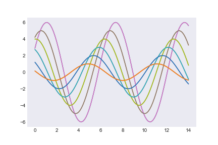
It’s a pretty basic set of sine curves, and while it looks pretty professional and clean, it doesn’t really tell us much more about what makes Seaborn unique. So what makes Seaborn different?
What are the benefits of Seaborn?
Well, let’s take a look at what Seaborn refers to as ‘joint plots.’ These plots pair a scatter plot with the distribution of each variable in the scatter plot on the axes. Let’s look at the code for the next two graphs and then we’ll discuss why they matter:
join1 = sns.jointplot(x="x", y="y", data=df);
join1.savefig("join1.png")
join2= sns.jointplot(x="x", y="y", data=df, kind="kde");
join2.savefig("join2.png")
plt.clf()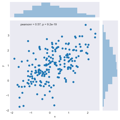
This plot isn’t unique to Seaborn. I’ve created very similar plots in R, however, that plot took one single line of code. In R, at the very least you’re looking at five or six lines, and you’re going to have to use the default plotting package because I’ve never been able to figure out marginal plots in ggplot2. Graphs like this really show us a lot about the data we are examining. We can simultaneously see that the two sets of data are correlated and that they are both somewhat skewed and non-normal, although the y variable could probably pass as normal. If marginal plots were this easy in R, I would leverage them a whole lot more because they are informative. The next plot, however, is different. In fact, I hadn’t really seen something like it before I learned about Seaborn.
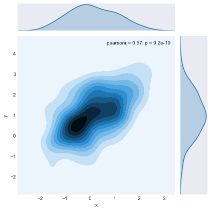
This plot uses a kernel density plot instead of a scatter plot, and the distributions are estimated smoothly instead of using histograms. This could be a helpful graph if you were specifically interested in densities and correlations as well as the distributions of the data. This could be quite beneficial in various spatial analysis applications, as well as traditional statistical fields. The third join plot includes a regression line in the scatter plot as well as an assessment of the fit of the linear model used. The code used to produce this plot is below:
tips = sns.load_dataset('tips')
sns.jointplot(x="total_bill", y="tip", data=tips, kind="reg");
plt.savefig('join3.png')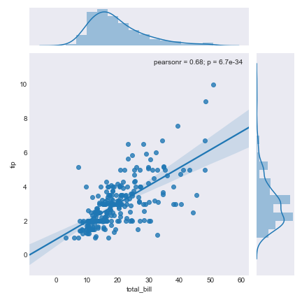
The inclusion of error fields around the line helps you to better visualize the accuracy of the linear regression. Additionally, the distribution of the data is available in the margins. Normally, it would take three separate graphs to convey all of this information. Seaborn makes this much simpler. With a single line of code, we are able to create a graph that covers all of the relevant information related to this linear regression.
Another somewhat novel graph type that’s available in Seaborn is the violin plot. Again, we can create this complex graph with the simple code shown below:
iris = sns.load_dataset("iris")
sns.violinplot(x=iris.species, y=iris.sepal_length, data=iris);
plt.savefig("violin.png")
This is data from the famous Iris data set. The violin plot is essentially an amalgamation of a box plot and a kernel density estimate of a distribution. Both box plots and graphs of univariate distributions are very helpful when first beginning analysis of some dataset. Again, Seaborn takes a lot out of the work of this process by making it easy to produce single graphs that would normally take multiple graphs using other analysis tools.

The final chart I would like to show is really useful. It summarizes the results of univariate logistic regression graphically. This is a tough thing to display and until I came across Seaborn I had really never seen an example I would consider good. The chart is created with the code below:
tips['big_tip'] = tips['tip']/tips['total_bill'] >= 0.2
sns.lmplot(x="total_bill", y="big_tip", data=tips,logistic=True, y_jitter=.03);
plt.savefig("tiplogit.png")
The chart displays the results of the regression a binary indicator if a tip was larger than 20 percent or ‘big’ against the total cost of the meal: 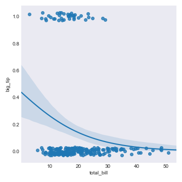
The chart illustrates very clearly that people are not tipping as much when their meals are more expensive, at least in terms of proportions. Summarizing the results of logistic regressions is always challenging, but as you can see, thanks to Seaborn, you can do a pretty good job with just one line of code.
Seaborn is simply a really great library that’s worth your time exploring – I hope this post has convinced you and inspired you to go and try it for yourself if you haven’t already. There is always room for improvement when it comes to data visualization. Seaborn might be the improvement you need. I know I’ll be using it.