In this article by Param Jeet and Prashant Vats, the author of the book Learning Quantitative Finance with R, will discuss about the types of regression and how we can build regression model in R for building predictive models. Also, how we can implement variable selection method and other aspects associated with regression. This article will not contain the theoretical description but it will just guide you how to implement regression model in R in financial space. Regression analysis can be used for doing forecast on cross-sectional data in financial domain.

This article covers the following topics:

• Simple linear regression
• Multivariate linear regression
• Multicollinearity
• ANOVA

(For more resources related to this topic, see here.)

Simple linear regression

In simple linear regression we try to predict one variable in terms of second variable called predictor variable. The variable we are trying to predict is called dependent variable and is denoted by y and the independent variable is denoted by x. In simple linear regression we assume linear relationship between dependent attribute and predictor attribute.

First we need to plot the data to understand the linear relationship between the dependent variable and independent variable. Here our data consists of two variables:

• YPrice: Dependent variable
• XPrice: Predictor variable

In this case we are trying to predict Yprice in terms of XPrice. StockXprice is independent variable and StockYprice is dependent variable. For every element of StockXprice there is an element of StockYprice which implies one to one mapping between elements of StockXprice and StockYprice.

Few lines of data used for the following analysis is displayed using the following code:

>head(Data)

	StockYPrice	StockXPrice
1	80.13	72.86
2	79.57	72.88
3	79.93	71.72
4	81.69	71.54
5	80.82	71
6	81.07	71.78

Scatter plot

First we will plot scatter plot between y and x to understand the type of linear relationship between x and y. The given followig code when executed, gives the following scatterplot:

> YPrice = Data$StockYPrice
> XPrice = Data$StockXPrice
> plot(YPrice, XPrice,       xlab=“XPrice“,        
ylab=“YPrice“)

Here our dependent variable is YPrice and predictor variable is Xprice. Please note this example is just for illustration purpose:

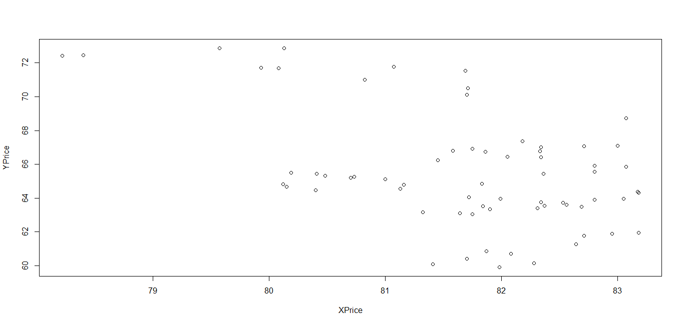Figure 3.1. Scatter plot of two variables

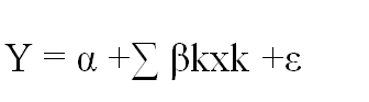
Once we examined the relationship between the dependent variable and predictor variable we try fit best straight line through the points which represents the predicted Y value for all the given predictor variable. A simple linear regression is represented by the following equation describing the relationship between the dependent and predictor variable:

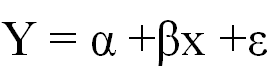
Where α and β are parameters and ε is error term. Whereα is also known as intercept and β as coefficient of predictor variable and is obtained by minimizing the sum of squares of error term ε. All the statistical software gives the option of estimating the coefficients and so does R.

We can fit the linear regression model using lm function in R as shown here:

> LinearR.lm = lm(YPrice ~ XPrice, data=Data)

Where Data is the input data given and Yprice and Xprice is the dependent and predictor variable respectively. Once we have fit the model we can extract our parameters using the following code:

> coeffs = coefficients(LinearR.lm); coeffs

The preceding resultant gives the value of intercept and coefficient:

(Intercept)      XPrice
92.7051345  -0.1680975

So now we can write our model as:

> YPrice = 92.7051345 + -0.1680975*(Xprice)

This can give the predicted value for any given Xprice.

Also, we can execute the given following code to get predicted value using the fit linear regression model on any other data say OutofSampleData by executing the following code:

> predict(LinearR.lm, OutofSampleData)

Coefficient of determination

We have fit our model but now we need to test how good the model is fitting to the data. There are few measures available for it but the main is coefficient of determination. This is given by the following code:

> summary(LinearR.lm)$r.squared

By definition, it is proportion of the variance in the dependent variable that is explained by the independent variable and is also known as R2.

Significance test

Now we need to examine that the relationship between the variables in linear regression model is significant or not at 0.05 significance level.

When we execute the following code will look like:

> summary(LinearR.lm)

It gives all the relevant statistics of the linear regression model as shown here:

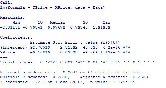Figure 3.2: Summary of linear regression model

If the Pvalue associated with Xprice is less than 0.05 then the predictor is explaining the dependent variable significantly at 0.05 significance level.

Confidence interval for linear regression model

One of the important issues for the predicted value is to find the confidence interval around the predicted value. So let us try to find 95% confidence interval around predicted value of the fit model. This can be achieved by executing the following code:

> Predictdata = data.frame(XPrice=75)

> predict(LinearR.lm, Predictdata, interval=“confidence“) 

Here we are estimating the predicted value for given value of Xprice = 75 and then the next we try to find the confidence interval around the predicted value.

The output generated by executing the preceding code is shown in the following screenshot::

Figure 3.3: Prediction of confidence interval for linear regression model

Residual plot

Once we have fitted the model then we compare it with the observed value and find the difference which is known as residual. Then we plot the residual against the predictor variable to see the performance of model visually. The following code can be executed to get the residual plot:

> LinearR.res = resid(LinearR.lm)
> plot(XPrice, LinearR.res, 
ylab=“Residuals“, xlab=“XPrice“, 
main=“Residual Plot“)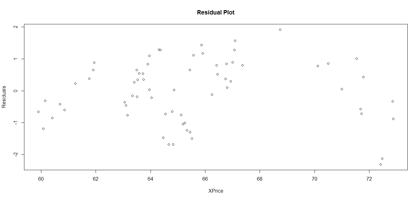

Figure 3.4: Residual plot of linear regression model

We can also plot the residual plot for standardized residual by just executing the following code in the previous mentioned code:

> LinearRSTD.res = rstandard(LinearR.lm)
> plot(XPrice, LinearRSTD.res, 
ylab=“Standardized Residuals“, xlab=“XPrice“, 
main=“Residual Plot“)

Normality distribution of errors

One of the assumption of linear regression is that errors are normally distributed and after fitting the model we need to check that errors are normally distributed.

Which can be checked by executing the following code and can be compared with theoretical normal distribution:

> qqnorm(LinearRSTD.res, 
ylab=“Standardized Residuals“, 
xlab=“Normal Scores“, 
main=“Error Normal Distribution plot“) 
> qqline(LinearRSTD.res)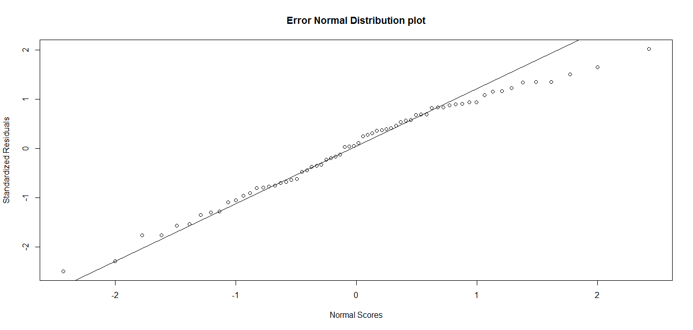

Figure 3.5: QQ plot of standardized residuals

Further detail of the summary function for linear regression model can be found in the R documentation. The following command will open a window which has complete information about linear regression model, that is, lm(). It also has information about each and every input variable including their data type, what are all the variable this function returns and how output variables can be extracted along with the examples:

> help(summary.lm) 

Multivariate linear regression

In multiple linear regression, we try to explain the dependent variable in terms of more than one predictor variable. The multiple linear regression equation is given by the following formula:

Where α, β1 …βk are multiple linear regression parameters and can be obtained by minimizing the sum of squares which is also known as OLS method of estimation.

Let us an take an example where we have the dependent variable StockYPrice and we are trying to predict it in terms of independent variables StockX1Price, StockX2Price, StockX3Price, StockX4Price, which is present in dataset DataMR.

Now let us fit the multiple regression model and get parameter estimates of multiple regression:

> MultipleR.lm = lm(StockYPrice ~  StockX1Price + StockX2Price +  StockX3Price + StockX4Price,  data=DataMR)
> summary(MultipleR.lm)

When we executed the preceding code, it fits the multiple regression model on the data and gives the basic summary of statistics associated with the multiple regression:

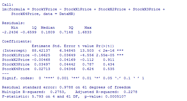Figure 3.6: Summary of multivariate linear regression

Just like simple linear regression model the lm function estimates the coefficients of multiple regression model as shown in the previous summary and we can write our prediction equation as follows:

> StockYPrice = 88.42137 +(-0.16625)*StockX1Price 
+ (-0.00468) * StockX2Price + (.03497)*StockX3Price+ (.02713)*StockX4Price

For any given set of independent variable we can find the predicted dependent variable by using the previous equation.

For any out of sample data we can obtain the forecast by executing the following code:

> newdata = data.frame(StockX1Price=70, StockX2Price=90, StockX3Price=60, StockX4Price=80)
> predict(MultipleR.lm, newdata)

Which gives the output 80.63105 as the predicted value of dependent variable for given set of independent variables.

Coefficient of determination

For checking the adequacy of model the main statistics is coefficient of determination and adjusted coefficient of determination which has been displayed in the summary table as R-Squared and Adjusted R-Squared matrices.

Also we can obtain them by the following code:

> summary(MultipleR.lm)$r.squared 

> summary(MultipleR.lm)$adj.r.squared 

From the summary table we can see which variables are coming significant. If the Pvalue associated with the variables in the summary table are <0.05 then the specific variable is significant, else it is insignificant.

Confidence interval

We can find the prediction interval for 95% confidence interval for the predicted value by multiple regression model by executing the following code:

> predict(MultipleR.lm, newdata, interval=“confidence“)

The following code generates the following output:

 Figure 3.7: Prediction of confidence interval for multiple regression model

Multicollinearity

If the predictor variables are correlated then we need to detect multicollinearity and treat it. Recognition of multicollinearity is very crucial because two of more variables are correlated which shows strong dependence structure between those variables and we are using correlated variables as independent variables which end up having double effect of these variables on the prediction because of relation between them. If we treat the multicollinearity and consider only variables which are not correlated then we can avoid the problem of double impact.

We can find multicollinearity by executing the following code:

> vif(MultipleR.lm)

This gives the multicollinearity table for the predictor variables:

 Figure 3.8: VIF table for multiple regression model

Depending upon the values of VIF we can drop the irrelevant variable.

ANOVA

ANOVA is used to determine whether there are any statistically significant differences between the means of three or more independent groups. In case of only two samples we can use the t-test to compare the means of the samples but in case of more than two samples it may be very complicated. We are going to study the relationship between a quantitative dependent variable returns and single qualitative independent variable stock. We have five levels of stock stock1, stock2, .. stock5.

We can study the four levels of stocks by means of boxplot and we can compare by executing the following code:

> DataANOVA = read.csv(“C:/Users/prashant.vats/Desktop/Projects/BOOK R/DataAnova.csv“)
>head(DataANOVA)

This displays few lines of the data used for analysis in the tabular format:

	Returns	Stock
1	1.64	Stock1
2	1.72	Stock1
3	1.68	Stock1
4	1.77	Stock1
5	1.56	Stock1
6	1.95	Stock1

>boxplot(DataANOVA$Returns ~ DataANOVA$Stock)

This gives the following output and boxplot it:

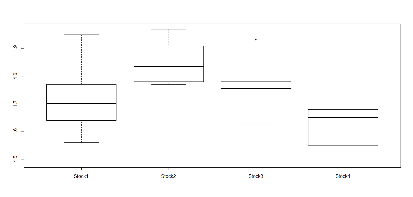Figure 3.9: Boxplot of different levels of stocks

The preceding boxplot shows that level stock has higher returns. If we repeat the procedure we are most likely going to get different returns. It may be possible that all the levels of stock gives similar numbers and we are just seeing random fluctuation in one set of returns. Let us assume that there is no difference at any level and it be our null hypothesis. Using ANOVA, let us test the significance of hypothesis:

> oneway.test(Returns ~ Stock, var.equal=TRUE)

Executing the preceding code gives the following outcome:

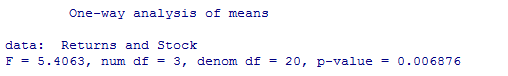Figure 3.10: Output of ANOVA for different levels of Stocks

Since Pvalue is less than 0.05 so the null hypothesis gets rejected. The returns at the different levels of stocks are not similar.

Summary

This article has been proven very beneficial to know some basic quantitative implementation with R. Moreover, you will also get to know the information regarding the packages that R use.

Resources for Article:

---

Further resources on this subject:

• What is Quantitative Finance? [article]
• Stata as Data Analytics Software [article]
• Using R for Statistics, Research, and Graphics [article]

---