


A neural network is made up of many artificial neurons. Is it a representation of the brain or is it a mathematical representation of some knowledge? Here, we will simply try to understand how a neural network is used in practice. A convolutional neural network (CNN) is a very special kind of multi-layer neural network. CNN is designed to recognize visual patterns directly from images with minimal processing. A graphical representation of this network is produced in the following image. The field of neural networks was originally inspired by the goal of modeling biological neural systems, but since then it has branched in different directions and has become a matter of engineering and attaining good results in machine learning tasks. In this article we will look at building blocks of neural networks and build a neural network which will recognize handwritten numbers in Keras and MNIST from 0-9.
This article is an excerpt taken from the book Practical Convolutional Neural Networks, written by Mohit Sewak, Md Rezaul Karim and Pradeep Pujari and published by Packt Publishing.
An artificial neuron is a function that takes an input and produces an output. The number of neurons that are used depends on the task at hand. It could be as low as two or as many as several thousands. There are numerous ways of connecting artificial neurons together to create a CNN. One such topology that is commonly used is known as a feed-forward network:
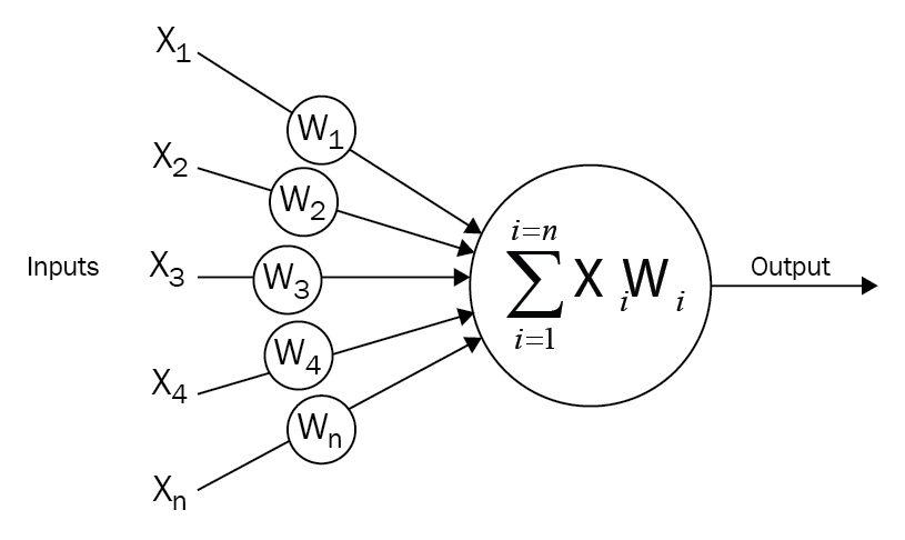
Each neuron receives inputs from other neurons. The effect of each input line on the neuron is controlled by the weight. The weight can be positive or negative. The entire neural network learns to perform useful computations for recognizing objects by understanding the language. Now, we can connect those neurons into a network known as a feed-forward network. This means that the neurons in each layer feed their output forward to the next layer until we get a final output. This can be written as follows:


The preceding forward-propagating neuron can be implemented as follows:
import numpy as np
import math

class Neuron(object):
   def __init__(self):
       self.weights = np.array([1.0, 2.0])
       self.bias = 0.0
   def forward(self, inputs):
       """ Assuming that inputs and weights are 1-D numpy arrays and the bias is a number """
       a_cell_sum = np.sum(inputs * self.weights) + self.bias
       result = 1.0 / (1.0 + math.exp(-a_cell_sum)) # This is the sigmoid activation function
       return result
neuron = Neuron()
output = neuron.forward(np.array([1,1]))
print(output)
Now that we have understood what are the building blocks of neural networks, let us get to building a neural network that will recognize handwritten numbers from 0 – 9.
Handwritten number recognition with Keras and MNIST
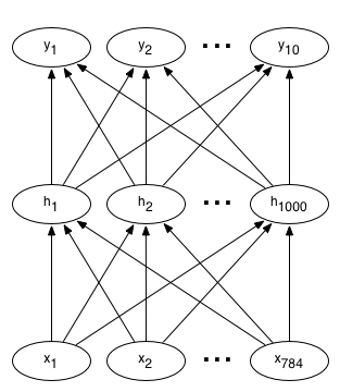
A typical neural network for a digit recognizer may have 784 input pixels connected to 1,000 neurons in the hidden layer, which in turn connects to 10 output targets — one for each digit. Each layer is fully connected to the layer above. A graphical representation of this network is shown as follows, where x are the inputs, h are the hidden neurons, and y are the output class variables:
In this notebook, we will build a neural network that will recognize handwritten numbers from 0-9.
The type of neural network that we are building is used in a number of real-world applications, such as recognizing phone numbers and sorting postal mail by address. To build this network, we will use the MNIST dataset.
We will begin as shown in the following code by importing all the required modules, after which the data will be loaded, and then finally building the network:
# Import Numpy, keras and MNIST dataimportnumpyasnpimportmatplotlib.pyplotaspltfromkeras.datasetsimportmnistfromkeras.modelsimportSequentialfromkeras.layers.coreimportDense,Dropout,Activationfromkeras.utilsimportnp_utilsRetrieving training and test data
The MNIST dataset already comprises both training and test data. There are 60,000 data points of training data and 10,000 points of test data. If you do not have the data file locally at the ‘~/.keras/datasets/’ + path, it can be downloaded at this location.
Each MNIST data point has:
- An image of a handwritten digit
- A corresponding label that is a number from 0-9 to help identify the image
The images will be called, and will be the input to our neural network, X; their corresponding labels are y.
We want our labels as one-hot vectors. One-hot vectors are vectors of many zeros and one. It’s easiest to see this in an example. The number 0 is represented as [1, 0, 0, 0, 0, 0, 0, 0, 0, 0], and 4 is represented as [0, 0, 0, 0, 1, 0, 0, 0, 0, 0] as a one-hot vector.
Flattened data
We will use flattened data in this example, or a representation of MNIST images in one dimension rather than two can also be used. Thus, each 28 x 28 pixels number image will be represented as a 784 pixel 1 dimensional array.
By flattening the data, information about the 2D structure of the image is thrown; however, our data is simplified. With the help of this, all our training data can be contained in one array of shape (60,000, 784), wherein the first dimension represents the number of training images and the second depicts the number of pixels in each image. This kind of data is easy to analyze using a simple neural network, as follows:
# Retrieving the training and test data
(X_train,y_train),(X_test,y_test)=mnist.load_data()
print('X_train shape:',X_train.shape)
print('X_test shape: ',X_test.shape)
print('y_train shape:',y_train.shape)
print('y_test shape: ',y_test.shape)
Visualizing the training data
The following function will help you visualize the MNIST data. By passing in the index of a training example, the show_digit function will display that training image along with its corresponding label in the title:
# Visualize the dataimportmatplotlib.pyplotasplt%matplotlibinline
#Displaying a training image by its index in the MNIST
setdefdisplay_digit(index):label=y_train[index].argmax(axis=0)image=X_train[index]plt.title('Training data, index: %d,  Label: %d'%(index,label))plt.imshow(image,cmap='gray_r')plt.show()# Displaying the first (index 0) training imagedisplay_digit(0)
X_train=X_train.reshape(60000,784)X_test=X_test.reshape(10000,784)X_train=X_train.astype('float32')X_test=X_test.astype('float32')X_train/=255X_test/=255print("Train the matrix shape",X_train.shape)print("Test the matrix shape",X_test.shape)

#One Hot encoding of
labels.fromkeras.utils.np_utilsimportto_categoricalprint(y_train.shape)y_train=to_categorical(y_train,10)y_test=to_categorical(y_test,10)print(y_train.shape)
Building the network
For this example, you’ll define the following:
- The input layer, which you should expect for each piece of MNIST data, as it tells the network the number of inputs
- Hidden layers, as they recognize patterns in data and also connect the input layer to the output layer
- The output layer, as it defines how the network learns and gives a label as the output for a given image, as follows:
# Defining the neural networkdefbuild_model():model=Sequential()model.add(Dense(512,input_shape=(784,)))model.add(Activation(‘relu’))# An “activation” is just a non-linear function that is applied to the output# of the above layer. In this case, with a “rectified linear unit”,# we perform clamping on all values below 0 to 0.model.add(Dropout(0.2))#With the help of Dropout helps we can protect the model from memorizing or “overfitting” the training datamodel.add(Dense(512))model.add(Activation(‘relu’))model.add(Dropout(0.2))model.add(Dense(10))model.add(Activation(‘softmax’))# This special “softmax” activation,#It also ensures that the output is a valid probability distribution,#Meaning that values obtained are all non-negative and sum up to 1.returnmodel
#Building the modelmodel=build_model()

model.compile(optimizer='rmsprop',loss='categorical_crossentropy',metrics=['accuracy'])
Training the network
Now that we’ve constructed the network, we feed it with data and train it, as follows:
# Trainingmodel.fit(X_train,y_train,batch_size=128,nb_epoch=4,verbose=1,validation_data=(X_test,y_test))Testing
After you’re satisfied with the training output and accuracy, you can run the network on the test dataset to measure its performance!
A good result will obtain an accuracy higher than 95%. Some simple models have been known to achieve even up to 99.7% accuracy! We can test the model, as shown here:
# Comparing the labels predicted by our model with the actual labelsscore=model.evaluate(X_test,y_test,batch_size=32,verbose=1,sample_weight=None)# Printing the resultprint('Test score:',score[0])print('Test accuracy:',score[1])To summarize we got to know about the building blocks of neural networks and we successfully built a neural network that recognized handwritten numbers using MNIST dataset in Keras. To implement award winning and cutting edge CNN architectures, check out this one stop guide published by Packtpub, Practical Convolutional Neural Networks.
Read Next:
Are Recurrent Neural Networks capable of warping time?
Recurrent neural networks and the LSTM architecture
Build a generative chatbot using recurrent neural networks (LSTM RNNs)


