


This is the second part of a two-part piece on Jupyter, a computing platform used by many scientists to perform their data analysis and modeling. This second part will dive into some code and give you a taste of what it is like to be a data scientist.
If you want to type along, you will need a Python installation with the following packages: the Jupyter-notebook (formerly the ipython notebook) and Python’s scientific stack. For installation instructions, see here or here. Go ahead and fire up the notebook by typing jupyter notebook into a command prompt, which will start a web server and point your browser to localhost:8888, and click on the button to create a new notebook backed by an IPython kernel.
The code for our first cell will be the following:
Cell 1:
%pylab inlineBy executing the cell (shift + enter), Jupyter will populate the namespace with various functions from the Numpy and Matplotlib packages as well as configuring the plotting engine to display figures as inline HTML images.
Output 1:
Populating the interactive namespace from numpy and matplotlibThe experiment
I’m a neuroscientist myself, so I’m going to show you a magic trick I once performed for my students. One student would volunteer to be equipped with an EEG cap and was put in front of a screen. On the screen, nine playing cards were presented to the volunteer with the instruction, “Pick any of these cards.”
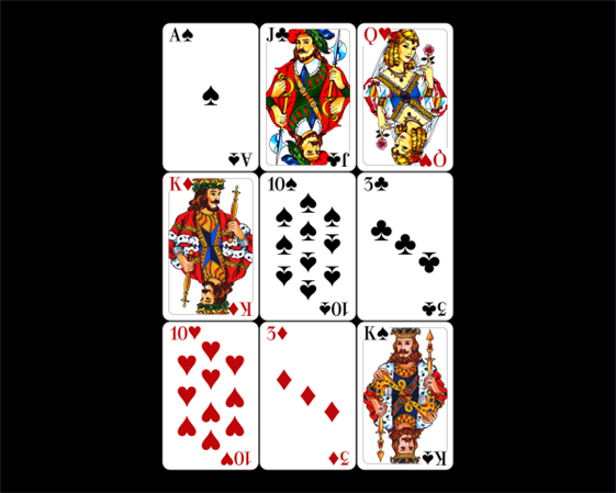
Image of the different cards that the volunteer could select
After the volunteer memorized the card, playing cards would flash across the screen one by one. The volunteer would mentally count the number of times his/her card was shown and not say anything to anyone. At the end of the sequence, I would analyze the EEG data and could tell with frightful accuracy which of the cards the volunteer had picked.
The secret to the trick is an EEG component called P300: a sharp peak in the signal when something grabs your attention (such as your card flashing across the screen).
The data
I’ve got a recording of myself as a volunteer; grab it here. It is stored as a MATLAB file, which can be loaded using SciPy’s loadmat function. The code will be the following.
Cell 2:
import scipy.io  # Import the IO module of SciPy

m = scipy.io.loadmat('tutorial1-01.mat')  # Load the MATLAB file

EEG = m['EEG']  # The EEG data stream
labels = m['labels'].flatten()  # Markers indicating when which card was shown

# The 9 possible cards the volunteer could have picked
cards = [
    'Ace of spades',
    'Jack of clubs',
    'Queen of hearts',
    'King of diamonds',
    '10 of spaces',
    '3 of clubs',
    '10 of hearts',
    '3 of diamonds',
    'King of spades',
]
The preceding code slaps the data onto our workbench. From here, we can use a huge assortment of tools to visualize and manipulate the data. The EEG and label variables are of the numpy.ndarray type, which is a data structure that is the bread and butter of data analysis in Python. It makes it easy to work with numeric data in the form of a multidimensional array. For example, we can query the size of the array via the following code.
Cell 3:
print 'EEG dimensions:', EEG.shape
print 'Label dimensions:', labels.shape
Output 3:
EEG dimensions: (7, 288349)
Label dimensions: (288349,)
I recorded EEG with seven electrodes, collecting numerous samples over time. Let’s visualize the EEG stream through the following code.
Cell 4:
figure(figsize=(15,3))   # Make a new figure of the given dimensions (in inches)
bases = 100 * arange(7)  # Add some vertical whitespace between the 7 channels
plot(EEG.T + bases)      # The .T property returns a version where rows and columns are transposed
xlabel('Time (samples)') # Label the X-axis, a good scientist always labels his/her axes!
Output 4:
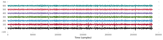
Output of cell 4
Note that NumPy’s arrays are very clever concerning arithmetical operators such as addition. Adding a single value to an array will add the value to each element in the array. Adding two equally sized arrays will sum up the corresponding elements. Adding a 1D array (a vector) to a 2D array (a matrix) will sum up the 1D array to every row of the 2D array. This is known as broadcasting and can save a ton of tedious for loops.
The labels variable is a 1D array that contains mostly zeros. However, on the exact onset of the presentation of a playing card, it contains the integer index (starting from 1) of the card being shown. Take a look at the following code.
Cell 5:
figure(figsize=(15,3))
scatter(arange(len(labels)), labels, edgecolor='white')  # Scatter plot
Output 5:
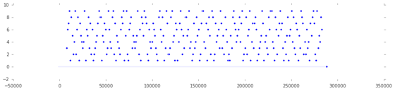
Output of cell 5
Slicing up the data
Cards were shown at a rate of two per second. We are interested in the response generated whenever a card was shown, so we cut one-second-long pieces of the EEG signal that starts from the moment a card was shown. These pieces will be named “trials”. A useful function here is flatnonzero, which returns all the indices of an array that contain a non-zero value. It effectively gives us the time (as an index) when a card was shown if we use it in a clever way. Execute the following code.
Cell 6:
# Get the onset of the presentation of each card
onsets = flatnonzero(labels)
print 'Onset of the first 10 cards:', onsets[:10]
print 'Total number of onsets:', len(onsets)

# Here is how we can use the onsets variable
classes = labels[onsets]
print 'First 10 cards shown:', classes[:10]
Output 6:
Onsers of the first 10 cards:[ 7789  8790  9814 10838 11862 12886 13910 14934 15958 16982]
Total number of onsets: 270
First 10 cards shown: [3 6 7 9 1 8 5 2 4 9]
In Line 7, we used another cool feature of NumPy’s arrays: fancy indexing. In addition to the classical indexing of an array using a single integer, we can index a NumPy array with another NumPy array as long as the second array contains only integers. Another useful way to index arrays is to use slices. Let’s use this to create a three-dimensional array containing all the trials. Take a look at the following code.
Cell 7:
nchannels = 7  # 7 EEG channels
sample_rate = 2048.  # The sample rate of the EEG recording device was 2048Hz
nsamples = int(1.0 * sample_rate) # one second's worth of data samples
ntrials = len(onsets)

trials = zeros((ntrials, nchannels, nsamples))
for i, onset in enumerate(onsets):
# Extract a slice of EEG data
    trials[i, :, :] = EEG[:, onset:onset + nsamples]

print trials.shape
Output 7:
(270, 7, 2048)We now have 270 trials (one trial for each time a card was flashed across the screen). Each trial consists of a little one-second piece of EEG recorded with seven channels using 2,048 samples. Let’s plot one of the trials by running the following code.
Cell 8:
figure(figsize=(4,4))
bases = 100 * arange(7)  # Add some vertical whitespace between the 7 channels
plot(trials[0, :, :].T + bases)
xlabel('Time (samples)')
Output 8:
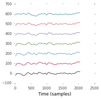
Output of cell 8
Reading my mind
Looking at the individual trials is not all that informative. Let’s calculate the average response to each card and plot it. To get all the trials where a particular card is shown, we can use the final way to index a NumPy array: using another array consisting of Boolean values. This is called Boolean or masked indexing. Take a look at the following code.
Cell 9:
# Lets give each response a different color
colors = ['k', 'b', 'g', 'y', 'm', 'r', 'c', '#ffff00', '#aaaaaa']

figure(figsize=(4,8))
bases = 20 * arange(7)  # Add some vertical whitespace between the 7 channels

# Plot the mean EEG response to each card, such an average is called an ERP in the literature
for i, card in enumerate(cards):
    # Use boolean indexing to get the right trial indices
    erp = mean(trials[classes == i+1, :, :], axis=0)
    plot(erp.T + bases, color=colors[i])
Output 9:
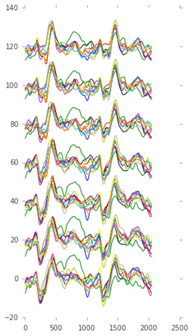
Output of cell 9
One of the cards jumps out: the one corresponding to the green line. This line corresponds to the third card, which turns out to be Queen of Hearts.
Yes, this was indeed the card I had picked!
Do you want to learn more?
This was a small taste of the pleasure it can be to manipulate data with modern tools such as Jupyter and Python’s scientific stack. To learn more, take a look at Numpy tutorial and Matplotlib tutorial. To learn even more, I recommend Cyrille Rossant’s IPython Interactive Computing and Visualization Cookbook.
About the author
Marijn van Vliet is a postdoctoral researcher at the department of Neuroscience and Biomedical Engineering at Aalto University. He uses Jupyter to analyse EEG and MEG recordings of the human brain in order to understand more about it processes written and spoken language. He can be found on Twitter @wmvanvliet.