


This tutorial will focus on some of the important architectures present today in deep learning. A lot of the success of neural networks lies in the careful design of the neural network architecture. We will look at the architecture of Autoencoder Neural Networks, Variational Autoencoders, CNN’s and RNN’s.
This tutorial is an excerpt from a book written by Dipanjan Sarkar, Raghav Bali, Et al titled Hands-On Transfer Learning with Python. This book extensively focuses on deep learning (DL) and transfer learning, comparing and contrasting the two with easy-to-follow concepts and examples.
Autoencoder neural networks
Autoencoders are typically used for reducing the dimensionality of data in neural networks. They are also successfully used for anomaly detection and novelty detection problems. Autoencoder neural networks come under the unsupervised learning category.
The network is trained by minimizing the difference between input and output. A typical autoencoder architecture is a slight variant of the DNN architecture, where the number of units per hidden layer is progressively reduced until a certain point before being progressively increased, with the final layer dimension being equal to the input dimension. The key idea behind this is to introduce bottlenecks in the network and force it to learn a meaningful compact representation. The middle layer of hidden units (the bottleneck) is basically the dimension-reduced encoding of the input. The first half of the hidden layers is called the encoder, and the second half is called the decoder. The following depicts a simple autoencoder architecture. The layer named z is the representation layer here:
 Source: cloud4scieng.org
Variational autoencoders
The variational autoencoders (VAEs) are generative models and compared to other deep generative models, VAEs are computationally tractable and stable and can be estimated by the efficient backpropagation algorithm. They are inspired by the idea of variational inference in Bayesian analysis.
The idea of variational inference is as follows: given input distribution x, the posterior probability distribution over output y is too complicated to work with. So, let’s approximate that complicated posterior, p(y | x), with a simpler distribution, q(y). Here, q is chosen from a family of distributions, Q, that best approximates the posterior. For example, this technique is used in training latent Dirichlet allocation (LDAs) (they do topic modeling for text and are Bayesian generative models).
Given a dataset, X, VAE can generate new samples similar but not necessarily equal to those in X. Dataset X has N Independent and Identically Distributed (IID) samples of some continuous or discrete random variable, x. Let’s assume that the data is generated by some random process, involving an unobserved continuous random variable, z. In this example of a simple autoencoder, the variable z is deterministic and is a stochastic variable. Data generation is a two-step process:
- A value of z is generated from a prior distribution, ρθ(z)
- A value of x is generated from the conditional distribution, ρθ(x|z)
So, p(x) is basically the marginal probability, calculated as:

The parameter of the distribution, θ, and the latent variable, z, are both unknown. Here, x can be generated by taking samples from the marginal p(x). Backpropagation cannot handle stochastic variable z or stochastic layer z within the network. Assuming the prior distribution, p(z), is Gaussian, we can leverage the location-scale property of Gaussian distribution, and rewrite the stochastic layer as z = μ + σε , where μ is the location parameter, σ is the scale, and ε is the white noise. Now we can obtain multiple samples of the noise, ε, and feed them as the deterministic input to the neural network.
Then, the model becomes an end-to-end deterministic deep neural network, as shown here:

Here, the decoder part is same as in the case of the simple autoencoder that we looked at earlier.
Types of CNN architectures
CNNs are multilayered neural networks designed specifically for identifying shape patterns with a high degree of invariance to translation, scaling, and rotation in two-dimensional image data. These networks need to be trained in a supervised way. Typically, a labeled set of object classes, such as MNIST or ImageNet, is provided as a training set. The crux of any CNN model is the convolution layer and the subsampling/pooling layer.
LeNet architecture
This is a pioneering seven-level convolutional network, designed by LeCun and their co-authors in 1998, that was used for digit classification. Later, it was applied by several banks to recognize handwritten numbers on cheques. The lower layers of the network are composed of alternating convolution and max pooling layers.
The upper layers are fully connected, dense MLPs (formed of hidden layers and logistic regression). The input to the first fully connected layer is the set of all the feature maps of the previous layer:

AlexNet
In 2012, AlexNet significantly outperformed all the prior competitors and won the ILSVRC by reducing the top-5 error to 15.3%, compared to the runner-up with 26%. This work popularized the application of CNNs in computer vision. AlexNet has a very similar architecture to that of LeNet, but has more filters per layer and is deeper. Also, AlexNet introduces the use of stacked convolution, instead of always using alternative convolution pooling. A stack of small convolutions is better than one large receptive field of convolution layers, as this introduces more non-linearities and fewer parameters.
ZFNet
The ILSVRC 2013 winner was a CNN from Matthew Zeiler and Rob Fergus. It became known as ZFNet. It improved on AlexNet by tweaking the architecture hyperparameters, in particular by expanding the size of the middle convolutional layers and making the stride and filter size on the first layer smaller, going from 11 x 11 stride 4 in AlexNet to 7 x 7 stride 2 in ZFNet. The intuition behind this was that a smaller filter size in the first convolution layer helps to retain a lot of the original pixel information. Also, AlexNet was trained on 15 million images, while ZFNet was trained on only 1.3 million images:

GoogLeNet (inception network)
The ILSVRC 2014 winner was a convolutional network called GoogLeNet from Google. It achieved a top-5 error rate of 6.67%! This was very close to human-level performance. The runner up was the network from Karen Simonyan and Andrew Zisserman known as VGGNet. GoogLeNet introduced a new architectural component using a CNN called the inception layer. The intuition behind the inception layer is to use larger convolutions, but also keep a fine resolution for smaller information on the images.
The following diagram describes the full GoogLeNet architecture:

Visual Geometry Group
Researchers from the Oxford Visual Geometry Group, or the VGG for short, developed the VGG network, which is characterized by its simplicity, using only 3 x 3 convolutional layers stacked on top of each other in increasing depth. Reducing volume size is handled by max pooling. At the end, two fully connected layers, each with 4,096 nodes, are then followed by a softmax layer. The only preprocessing done to the input is the subtraction of the mean RGB value, computed on the training set, from each pixel.
Pooling is carried out by max pooling layers, which follow some of the convolution layers. Not all the convolution layers are followed by max pooling. Max pooling is performed over a 2 x 2 pixel window, with a stride of 2. ReLU activation is used in each of the hidden layers. The number of filters increases with depth in most VGG variants. The 16-layered architecture VGG-16 is shown in the following diagram. The 19-layered architecture with uniform 3 x 3 convolutions (VGG-19) is shown along with ResNet in the following section. The success of VGG models confirms the importance of depth in image representations:
 VGG-16: Input RGB image of size 224 x 224 x 3, the number of filters in each layer is circled
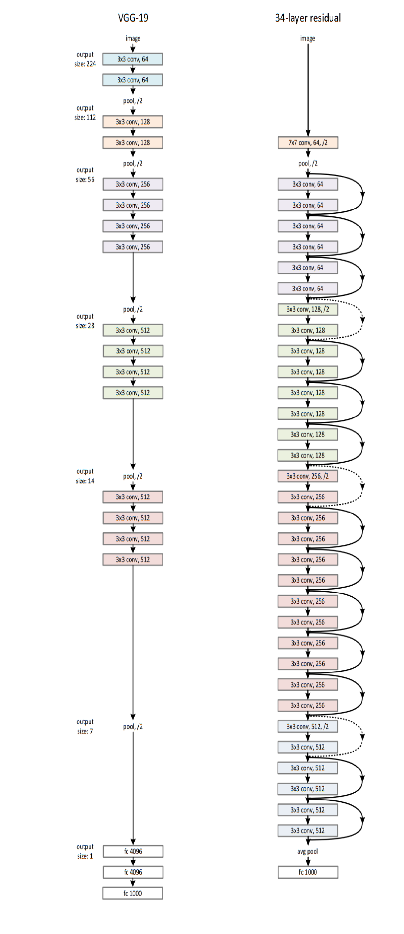
Residual Neural Networks
The main idea in this architecture is as follows. Instead of hoping that a set of stacked layers would directly fit a desired underlying mapping, H(x), they tried to fit a residual mapping. More formally, they let the stacked set of layers learn the residual R(x) = H(x) – x, with the true mapping later being obtained by a skip connection. The input is then added to the learned residual, R(x) + x.
Also, batch normalization is applied right after each convolution and before activation:

Here is the full ResNet architecture compared to VGG-19. The dotted skip connections show an increase in dimensions; hence, for the addition to be valid, no padding is done. Also, increases in dimensions are indicated by changes in color:
Types of RNN architectures
An recurrent neural Network (RNN) is specialized for processing a sequence of values, as in x(1), . . . , x(t). We need to do sequence modeling if, say, we wanted to predict the next term in the sequence given the recent history of the sequence, or maybe translate a sequence of words in one language to another language. RNNs are distinguished from feedforward networks by the presence of a feedback loop in their architecture. It is often said that RNNs have memory. The sequential information is preserved in the RNNs hidden state. So, the hidden layer in the RNN is the memory of the network. In theory, RNNs can make use of information in arbitrarily long sequences, but in practice they are limited to looking back only a few steps.
LSTMs
RNNs start losing historical context over time in the sequence, and hence are hard to train for practical purposes. This is where LSTMs (Long short-term memory) come into the picture! Introduced by Hochreiter and Schmidhuber in 1997, LSTMs can remember information from really long sequence-based data and prevent issues such as the vanishing gradient problem. LSTMs usually consist of three or four gates, including input, output, and forget gates.
The following diagram shows a high-level representation of a single LSTM cell:

The input gate can usually allow or deny incoming signals or inputs to alter the memory cell state. The output gate usually propagates the value to other neurons as necessary. The forget gate controls the memory cell’s self-recurrent connection to remember or forget previous states as necessary. Multiple LSTM cells are usually stacked in any deep learning network to solve real-world problems, such as sequence prediction.
Stacked LSTMs
If we want to learn about the hierarchical representation of sequential data, a stack of LSTM layers can be used. Each LSTM layer outputs a sequence of vectors rather than a single vector for each item of the sequence, which will be used as an input to a subsequent LSTM layer. This hierarchy of hidden layers enables a more complex representation of our sequential data. Stacked LSTM models can be used for modeling complex multivariate time series data.
Encoder-decoder – Neural Machine Translation
Machine translation is a sub-field of computational linguistics, and is about performing translation of text or speech from one language to another. Traditional machine translation systems typically rely on sophisticated feature engineering based on the statistical properties of text. Recently, deep learning has been used to solve this problem, with an approach known as Neural Machine Translation (NMT). An NMT system typically consists of two modules: an encoder and a decoder.
It first reads the source sentence using the encoder to build a thought vector: a sequence of numbers that represents the sentence’s meaning. A decoder processes the sentence vector to emit a translation to other target languages. This is called an encoder-decoder architecture. The encoders and decoders are typically forms of RNN. The following diagram shows an encoder-decoder architecture using stacked LSTMs.
 Source: tensorflow.org
The source code for NMT in TensorFlow is available at Github.
Gated Recurrent Units
Gated Recurrent Units (GRUs) are related to LSTMs, as both utilize different ways of gating information to prevent the vanishing gradient problem and store long-term memory. A GRU has two gates: a reset gate, r, and an update gate, z, as shown in the following diagram. The reset gate determines how to combine the new input with the previous hidden state, ht-1, and the update gate defines how much of the previous state information to keep. If we set the reset to all ones and update gate to all zeros, we arrive at a simple RNN model:

GRUs are computationally more efficient because of a simpler structure and fewer parameters.
Summary
This article covered various advances in neural network architectures including Autoencoder Neural Networks, Variational Autoencoders, CNN’s and RNN’s architectures.
To understand how to simplify deep learning by taking supervised, unsupervised, and reinforcement learning to the next level using the Python ecosystem, check out this book Hands-On Transfer Learning with Python
Read Next
Neural Style Transfer: Creating artificial art with deep learning and transfer learning
Dr. Brandon explains ‘Transfer Learning’ to Jon
5 cool ways Transfer Learning is being used today


