


TensorFlow is a mathematical software and an open source framework for deep learning developed by the Google Brain Team in 2011. Nevertheless, it can be used to help us analyze data in order to predict an effective business outcome.
Although the initial target of TensorFlow was to conduct research in ML and in Deep Neural Networks (DNNs), the system is general enough to be applicable to a wide variety of classical machine learning algorithm such as Support Vector Machine (SVM), logistic regression, decision trees, random forest and so on.
In this article we will talk about data model in TensorFlow. The data model in TensorFlow is represented by tensors. Without using complex mathematical definitions, we can say that a tensor (in TensorFlow) identifies a multidimensional numerical array. We will see more details on tensors in the next subsection.
This article is taken from the book Deep Learning with TensorFlow – Second Edition by Giancarlo Zaccone and Md. Rezaul Karim. In this book, we will delve into neural networks, implement deep learning algorithms, and explore layers of data abstraction with the help of TensorFlow.
Tensors in a data model
Let’s see the formal definition of tensor on Wikipedia, as follows:
“Tensors are geometric objects that describe linear relations between geometric vectors, scalars, and other tensors. Elementary examples of such relations include the dot product, the cross product, and linear maps. Geometric vectors, often used in physics and engineering applications, and scalars themselves are also tensors.”
This data structure is characterized by three parameters: rank, shape, and type, as shown in the following figure:

Figure 6: Tensors are nothing but geometric objects with a shape, rank, and type, used to hold a multidimensional array
A tensor can thus be thought of as the generalization of a matrix that specifies an element with an arbitrary number of indices. The syntax for tensors is more or less the same as nested vectors.
[box type=”shadow” align=”” class=”” width=””]Tensors just define the type of this value and the means by which this value should be calculated during the session. Therefore, they do not represent or hold any value produced by an operation.[/box]
Some people love to compare NumPy and TensorFlow. However, in reality, TensorFlow and NumPy are quite similar in the sense that both are N-d array libraries!
Well, it’s true that NumPy has n-dimensional array support, but it doesn’t offer methods to create tensor functions and automatically compute derivatives (and it has no GPU support). The following figure is a short and one-to-one comparison of NumPy and TensorFlow:
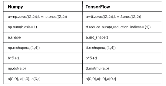
Figure 7: NumPy versus TensorFlow: a one-to-one comparison
Now let’s see an alternative way of creating tensors before they could be fed (we will see other feeding mechanisms later on) by the TensorFlow graph:
>>> X = [[2.0, 4.0],

       [6.0, 8.0]] # X is a list of lists

>>> Y = np.array([[2.0, 4.0],

             [6.0, 6.0]], dtype=np.float32)#Y is a Numpy array

>>> Z = tf.constant([[2.0, 4.0],

                [6.0, 8.0]]) # Z is a tensor
Here, X is a list, Y is an n-dimensional array from the NumPy library, and Z is a TensorFlow tensor object. Now let’s see their types:
>>> print(type(X))

>>> print(type(Y))

>>> print(type(Z))

#Output

<class 'list'>

<class 'numpy.ndarray'>

<class 'tensorflow.python.framework.ops.Tensor'>
Well, their types are printed correctly. However, a more convenient function that we’re formally dealing with tensors as opposed to the other types is tf.convert_to_tensor() function as follows:
t1 = tf.convert_to_tensor(X, dtype=tf.float32)

t2 = tf.convert_to_tensor(Y dtype=tf.float32)

Now let's see their types using the following code:

>>> print(type(t1))

>>> print(type(t2))

#Output:

<class 'tensorflow.python.framework.ops.Tensor'>

<class 'tensorflow.python.framework.ops.Tensor'>
Fantastic! That’s enough discussion about tensors for now. So, we can think about the structure that is characterized by the term rank.
Rank and shape of Tensors
A unit of dimensionality called rank describes each tensor. It identifies the number of dimensions of the tensor. For this reason, a rank is known as order or n–dimensions of a tensor. A rank zero tensor is a scalar, a rank one tensor is a vector, and a rank two tensor is a matrix.
The following code defines a TensorFlow scalar, vector, matrix, and cube_matrix. In the next example, we will show how rank works:
import tensorflow as tf

scalar = tf.constant(100)

vector = tf.constant([1,2,3,4,5])

matrix = tf.constant([[1,2,3],[4,5,6]])

cube_matrix =

tf.constant([[[1],[2],[3]],[[4],[5],[6]],[[7],[8],[9]]])

print(scalar.get_shape())

print(vector.get_shape())

print(matrix.get_shape())

print(cube_matrix.get_shape())
The results are printed here:
>>>

()

(5,)

(2, 3)

(3, 3, 1)

>>>
The shape of a tensor is the number of rows and columns it has. Now we will see how to relate the shape of a tensor to its rank:
>>scalar.get_shape()

TensorShape([])

>>vector.get_shape()

TensorShape([Dimension(5)])

>>matrix.get_shape()

TensorShape([Dimension(2), Dimension(3)])

>>cube.get_shape()

TensorShape([Dimension(3), Dimension(3), Dimension(1)])
Data type of Tensors
In addition to rank and shape, tensors have a data type. Here is a list of the data types:
| Data type | Python type | Description |
| DT_FLOAT | tf.float32 | 32-bit floating point |
| DT_DOUBLE | tf.float64 | 64-bit floating point |
| DT_INT8 | tf.int8 | 8-bit signed integer |
| DT_INT16 | tf.int16 | 16-bit signed integer |
| DT_INT32 | tf.int32 | 32-bit signed integer |
| DT_INT64 | tf.int64 | 64-bit signed integer |
| DT_UINT8 | tf.uint8 | 8-bit unsigned integer |
| DT_STRING | tf.string | Variable length byte arrays. Each element of a tensor is a byte array |
| DT_BOOL | tf.bool | Boolean |
| DT_COMPLEX64 | tf.complex64 | Complex number made of two 32-bit floating points: real and imaginary parts |
| DT_COMPLEX128 | tf.complex128 | Complex number made of two 64-bit floating points: real and imaginary parts |
| DT_QINT8 | tf.qint8 | 8-bit signed integer used in quantized Ops |
| DT_QINT32 | tf.qint32 | 32-bit signed integer used in quantized Ops |
| DT_QUINT8 | tf.quint8 | 8-bit unsigned integer used in quantized Ops |
The preceding table is self-explanatory, so we have not provided a detailed discussion of the data types. The TensorFlow APIs are implemented to manage data to and from NumPy arrays.
Thus, to build a tensor with a constant value, pass a NumPy array to the tf.constant() operator, and the result will be a tensor with that value:
import tensorflow as tf

import numpy as np

array_1d = np.array([1,2,3,4,5,6,7,8,9,10])

tensor_1d = tf.constant(array_1d)

with tf.Session() as sess:

   print(tensor_1d.get_shape())

   print(sess.run(tensor_1d))
# Close the TensorFlow session when you’re done
sess.close()Running the example, we obtain the following:
>>>

(10,)

[ 1  2 3 4  5 6 7 8  9 10]
To build a tensor with variable values, use a NumPy array and pass it to the tf.Variable constructor. The result will be a variable tensor with that initial value:
import tensorflow as tf

import numpy as np

# Create a sample NumPy array

array_2d = np.array([(1,2,3),(4,5,6),(7,8,9)])

# Now pass the preceding array to tf.Variable()

tensor_2d = tf.Variable(array_2d)

# Execute the preceding op under an active session

with tf.Session() as sess:

   sess.run(tf.global_variables_initializer())

   print((tensor_2d.get_shape()))

   print sess.run(tensor_2d)
# Finally, close the TensorFlow session when you’re done
sess.close()In the preceding code block, tf.global_variables_initializer() is used to initialize all the ops we created before. If you need to create a variable with an initial value dependent on another variable, use the other variable’s initialized_value(). This ensures that variables are initialized in the right order.
The result is as follows:
>>>

(3, 3)

[[1 2 3]

[4 5 6]

[7 8 9]]
For ease of use in interactive Python environments, we can use the InteractiveSession class, and then use that session for all Tensor.eval() and Operation.run() calls:
import tensorflow as tf # Import TensorFlow

import numpy as np # Import numpy

# Create an interactive TensorFlow session

interactive_session = tf.InteractiveSession()

# Create a 1d NumPy array

array1 = np.array([1,2,3,4,5]) # An array

# Then convert the preceding array into a tensor

tensor = tf.constant(array1) # convert to tensor

print(tensor.eval()) # evaluate the tensor op

interactive_session.close() # close the session
[box type=”shadow” align=”” class=”” width=””]tf.InteractiveSession() is just convenient syntactic sugar for keeping a default session open in IPython.[/box]
The result is as follows:
>>>

  [1 2 3 4 5]
This can be easier in an interactive setting, such as the shell or an IPython Notebook, as it can be tedious to pass around a session object everywhere.
[box type=”shadow” align=”” class=”” width=””]The IPython Notebook is now known as the Jupyter Notebook. It is an interactive computational environment in which you can combine code execution, rich text, mathematics, plots, and rich media. For more information, interested readers should refer to https://ipython.org/notebook.html.[/box]
Another way to define a tensor is using the tf.convert_to_tensor statement:
import tensorflow as tf

import numpy as np

tensor_3d = np.array([[[0, 1, 2], [3, 4, 5], [6, 7, 8]],

                  [[9, 10, 11], [12, 13, 14], [15, 16, 17]],

                 [[18, 19, 20], [21, 22, 23], [24, 25, 26]]])

tensor_3d = tf.convert_to_tensor(tensor_3d, dtype=tf.float64)

with tf.Session() as sess:

   print(tensor_3d.get_shape())

   print(sess.run(tensor_3d))
# Finally, close the TensorFlow session when you’re done
sess.close()Following is the output of the preceding code:
>>>

(3, 3, 3)

[[[  0. 1.   2.]

 [ 3.   4. 5.]

 [ 6.   7. 8.]]

[[  9. 10.  11.]

 [ 12.  13. 14.]

 [ 15.  16. 17.]]

[[ 18.  19. 20.]

 [ 21.  22. 23.]

 [ 24.  25. 26.]]]
Variables
Variables are TensorFlow objects used to hold and update parameters. A variable must be initialized so that you can save and restore it to analyze your code later on. Variables are created by using either tf.Variable() or tf.get_variable() statements. Whereas tf.get_varaiable() is recommended but tf.Variable() is lower-label abstraction.
In the following example, we want to count the numbers from 1 to 10, but let’s import TensorFlow first:
import tensorflow as tf

We created a variable that will be initialized to the scalar value 0:

value = tf.get_variable("value", shape=[], dtype=tf.int32,

initializer=None, regularizer=None, trainable=True,

collections=None)
The assign() and add() operators are just nodes of the computation graph, so they do not execute the assignment until the session is run:
one = tf.constant(1)

update_value = tf.assign_add(value, one)

initialize_var = tf.global_variables_initializer()

We can instantiate the computation graph:

with tf.Session() as sess:

   sess.run(initialize_var)

   print(sess.run(value))

   for _ in range(5):

       sess.run(update_value)

       print(sess.run(value))

# Close the session

sess.close()
Let’s recall that a tensor object is a symbolic handle to the result of an operation, but it does not actually hold the values of the operation’s output:
>>>

0

1

2

3

4

5
Fetches
To fetch the output of an operation, the graph can be executed by calling run() on the session object and passing in the tensors. Apart from fetching a single tensor node, you can also fetch multiple tensors.
In the following example, the sum and multiply tensors are fetched together using the run() call:
import tensorflow as tf

constant_A = tf.constant([100.0])

constant_B = tf.constant([300.0])

constant_C = tf.constant([3.0])

sum_ = tf.add(constant_A,constant_B)

mul_ = tf.multiply(constant_A,constant_C)

with tf.Session() as sess:

   result = sess.run([sum_,mul_])# _ means throw away afterwards

   print(result)

# Finally, close the TensorFlow session when you're done:

sess.close()
The output is as follows:
>>>

[array(400.],dtype=float32),array([ 300.],dtype=float32)]
It should be noted that all the ops that need to be executed (that is, in order to produce tensor values) are run once (not once per requested tensor).
Feeds and placeholders
There are four methods of getting data into a TensorFlow program (for more information, see https://www.tensorflow.org/api_guides/python/reading_data):
The Dataset API: This enables you to build complex input pipelines from simple and reusable pieces of distributed filesystems and perform complex operations. Using the Dataset API is recommended if you are dealing with large amounts of data in different data formats. The Dataset API introduces two new abstractions to TensorFlow for creating a feedable dataset: tf.contrib.data.Dataset (by creating a source or applying transformation operations) and tf.contrib.data.Iterator.
Feeding: This allows us to inject data into any tensor in a computation graph.
Reading from files: This allows us to develop an input pipeline using Python’s built-in mechanism for reading data from data files at the beginning of the graph.
Preloaded data: For a small dataset, we can use either constants or variables in the TensorFlow graph to hold all the data.
In this section, we will see an example of a feeding mechanism. TensorFlow provides a feed mechanism that allows us to inject data into any tensor in a computation graph. You can provide the feed data through the feed_dict argument to a run() or eval() invocation that initiates the computation.
[box type=”shadow” align=”” class=”” width=””]Feeding using feed_dict argument is the least efficient way to feed data into a TensorFlow execution graph and should only be used for small experiments needing small dataset. It can also be used for debugging.[/box]
We can also replace any tensor with feed data (that is, variables and constants). Best practice is to use a TensorFlow placeholder node using tf.placeholder() (https://www.tensorflow.org/api_docs/python/tf/placeholder). A placeholder exists exclusively to serve as the target of feeds. An empty placeholder is not initialized, so it does not contain any data.
Therefore, it will always generate an error if it is executed without a feed, so you won’t forget to feed it. The following example shows how to feed data to build a random 2×3 matrix:
import tensorflow as tf

import numpy as np

a = 3

b = 2

x = tf.placeholder(tf.float32,shape=(a,b))

y = tf.add(x,x)

data = np.random.rand(a,b)

sess = tf.Session()

print(sess.run(y,feed_dict={x:data}))

sess.close()# close the session
The output is as follows:
>>>

[[ 1.78602004  1.64606333]

[ 1.03966308  0.99269408]

[ 0.98822606  1.50157797]]

>>>
We understood the data model in TensorFlow. To understand the TensorFlow computational graph and the TensorFlow code structure, read our book Deep Learning with TensorFlow – Second Edition.
Read Next
Why TensorFlow always tops machine learning and artificial intelligence tool surveys.


