TensorFlow is another open source library developed by the Google Brain Team to build numerical computation models using data flow graphs. The core of TensorFlow was developed in C++ with the wrapper in Python. The tensorflow package in R gives you access to the TensorFlow API composed of Python modules to execute computation models. TensorFlow supports both CPU- and GPU-based computations. In this article, we will cover the application of TensorFlow in setting up a logistic regression model. The example will use a similar dataset to that used in the H2O model setup.

The tensorflow package in R calls the Python tensorflow API for execution, which is essential to install the tensorflow package in both R and Python to make R work. The following are the dependencies for tensorflow:

• Python 2.7 / 3.x
• R (>3.2)
• devtools package in R for installing TensorFlow from GitHub
• TensorFlow in Python
• pip

Getting ready

The code for this section is created on Linux but can be run on any operating system. To start modeling, load the tensorflow package in the environment. R loads the default TensorFlow environment variable and also the NumPy library from Python in the np variable:

library("tensorflow") # Load TensorFlow 
np <- import("numpy") # Load numpy library

How to do it…

The data is imported using a standard function from R, as shown in the following code.

1. The data is imported using the csv file and transformed into the matrix format followed by selecting the features used to model as defined in xFeatures and yFeatures. The next step in TensorFlow is to set up a graph to run optimization:

# Loading input and test data
xFeatures = c("Temperature", "Humidity", "Light", "CO2", "HumidityRatio")
yFeatures = "Occupancy"
occupancy_train <-as.matrix(read.csv("datatraining.txt",stringsAsFactors = T))
occupancy_test <- as.matrix(read.csv("datatest.txt",stringsAsFactors = T))

# subset features for modeling and transform to numeric values
occupancy_train<-apply(occupancy_train[, c(xFeatures, yFeatures)], 2, FUN=as.numeric) 
occupancy_test<-apply(occupancy_test[, c(xFeatures, yFeatures)], 2, FUN=as.numeric)

# Data dimensions
nFeatures<-length(xFeatures)
nRow<-nrow(occupancy_train)

2. Before setting up the graph, let’s reset the graph using the following command:

# Reset the graph
tf$reset_default_graph()

3. Additionally, let’s start an interactive session as it will allow us to execute variables without referring to the session-to-session object:

# Starting session as interactive session
sess<-tf$InteractiveSession()

4. Define the logistic regression model in TensorFlow:

# Setting-up Logistic regression graph
x <- tf$constant(unlist(occupancy_train[, xFeatures]), shape=c(nRow, nFeatures), dtype=np$float32) # 
W <- tf$Variable(tf$random_uniform(shape(nFeatures, 1L)))
b <- tf$Variable(tf$zeros(shape(1L)))
y <- tf$matmul(x, W) + b

5. The input feature x is defined as a constant as it will be an input to the system. The weight W and bias b are defined as variables that will be optimized during the optimization process. The y is set up as a symbolic representation between x, W, and b. The weight W is set up to initialize random uniform distribution and b is assigned the value zero.
6. The next step is to set up the cost function for logistic regression:

# Setting-up cost function and optimizer
y_ <- tf$constant(unlist(occupancy_train[, yFeatures]), dtype="float32", shape=c(nRow, 1L))
cross_entropy<-tf$reduce_mean(tf$nn$sigmoid_cross_entropy_with_logits(labels=y_, logits=y, name="cross_entropy"))
optimizer <- tf$train$GradientDescentOptimizer(0.15)$minimize(cross_entropy)

# Start a session
init <- tf$global_variables_initializer()
sess$run(init)

7. Execute the gradient descent algorithm for the optimization of weights using cross entropy as the loss function:

# Running optimization 
for (step in 1:5000) {
  sess$run(optimizer)
  if (step %% 20== 0)
    cat(step, "-", sess$run(W), sess$run(b), "==>", sess$run(cross_entropy), "n")
}

How it works…

The performance of the model can be evaluated using AUC:

# Performance on Train
library(pROC) 
ypred <- sess$run(tf$nn$sigmoid(tf$matmul(x, W) + b))
roc_obj <- roc(occupancy_train[, yFeatures], as.numeric(ypred))

# Performance on test
nRowt<-nrow(occupancy_test)
xt <- tf$constant(unlist(occupancy_test[, xFeatures]), shape=c(nRowt, nFeatures), dtype=np$float32)
ypredt <- sess$run(tf$nn$sigmoid(tf$matmul(xt, W) + b))
roc_objt <- roc(occupancy_test[, yFeatures], as.numeric(ypredt)).

AUC can be visualized using the plot.auc function from the pROC package, as shown in the screenshot following this command. The performance for training and testing (hold-out) is very similar.

plot.roc(roc_obj, col = "green", lty=2, lwd=2)
plot.roc(roc_objt, add=T, col="red", lty=4, lwd=2)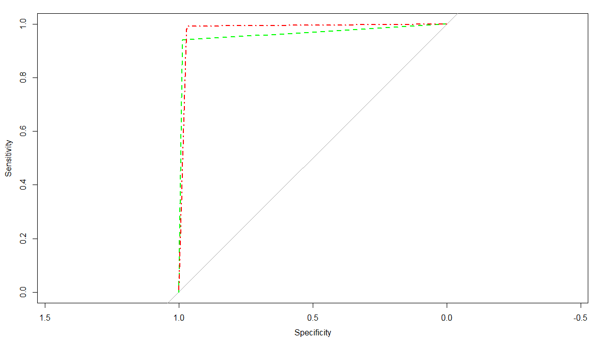

Performance of logistic regression using TensorFlow

Visualizing TensorFlow graphs

TensorFlow graphs can be visualized using TensorBoard. It is a service that utilizes TensorFlow event files to visualize TensorFlow models as graphs. Graph model visualization in TensorBoard is also used to debug TensorFlow models.

Getting ready

TensorBoard can be started using the following command in the terminal:

$ tensorboard --logdir home/log --port 6006

The following are the major parameters for TensorBoard:

• –logdir : To map to the directory to load TensorFlow events
• –debug: To increase log verbosity
• –host: To define the host to listen to its localhost (0.0.1) by default
• –port: To define the port to which TensorBoard will serve

The preceding command will launch the TensorFlow service on localhost at port 6006, as shown in the following screenshot:

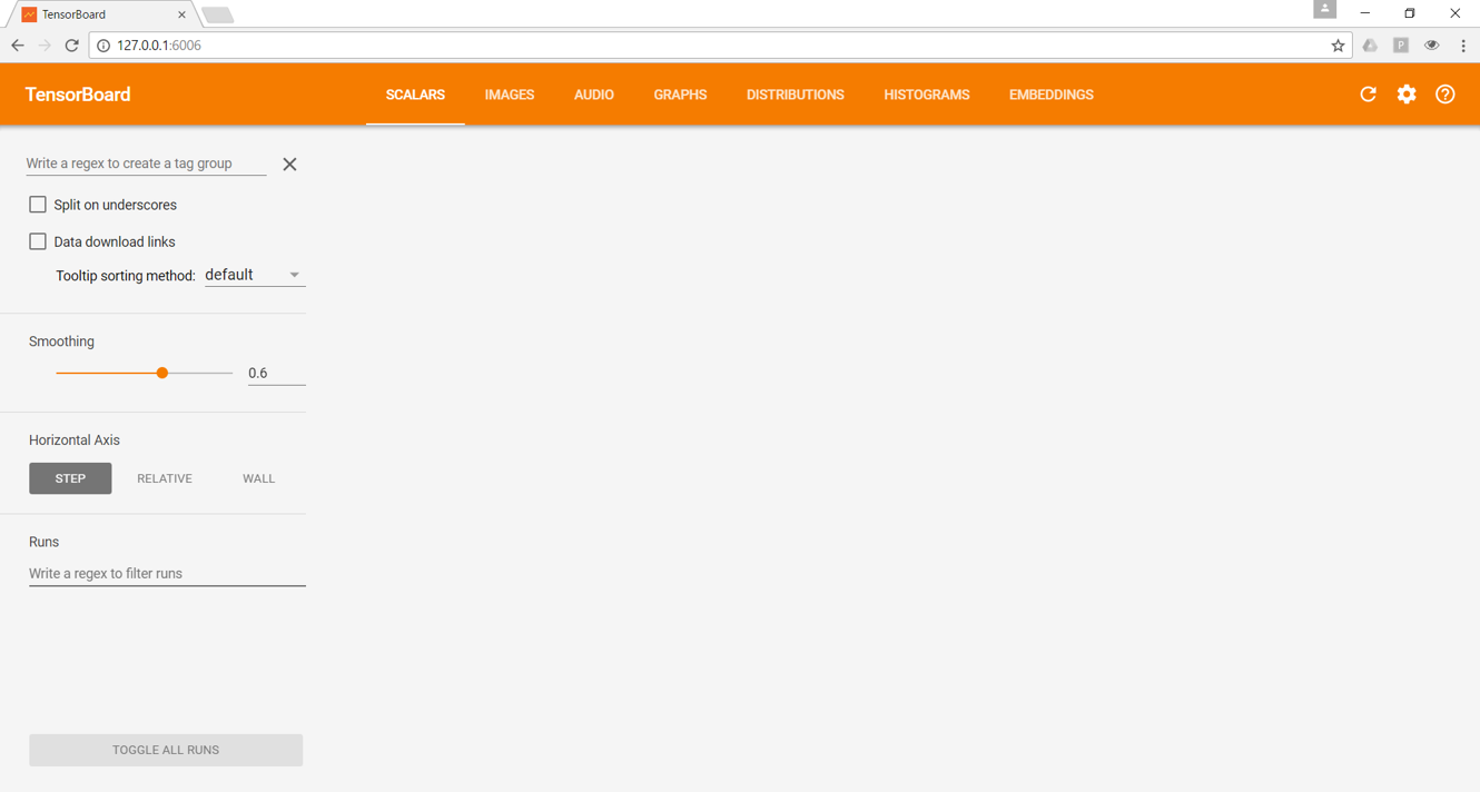
TensorBoard

The tabs on the TensorBoard capture relevant data generated during graph execution.

How to do it…

The section covers how to visualize TensorFlow models and output in TernsorBoard.

1. To visualize summaries and graphs, data from TensorFlow can be exported using the FileWriter command from the summary module. A default session graph can be added using the following command:

# Create Writer Obj for log
log_writer = tf$summary$FileWriter('c:/log', sess$graph)

The graph for logistic regression developed using the preceding code is shown in the following screenshot:

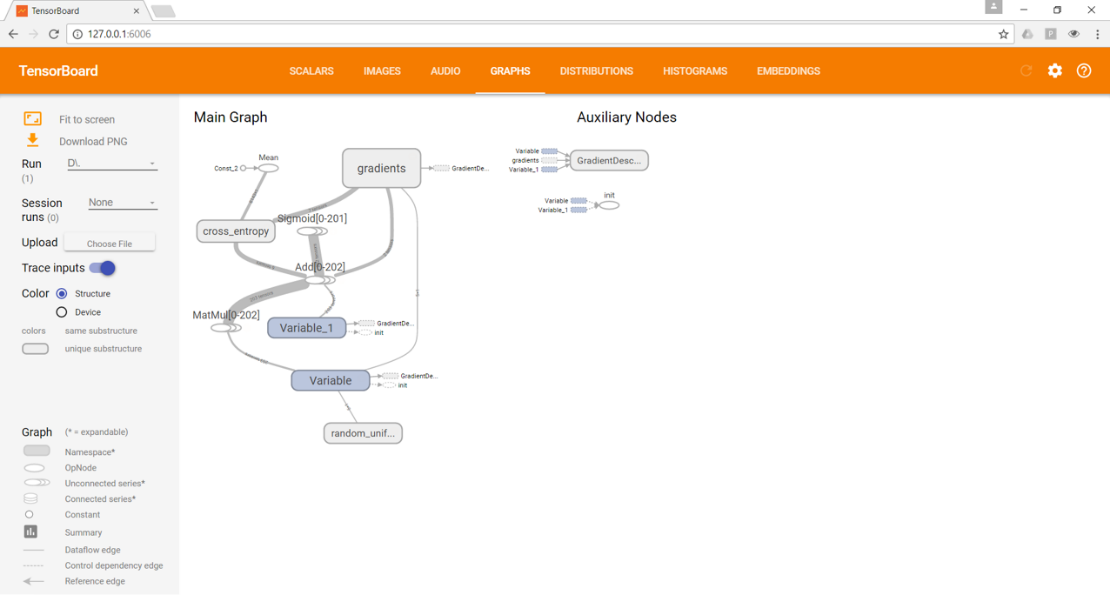
Visualization of the logistic regression graph in TensorBoard

Details about symbol descriptions on TensorBoard can be found at https://www.tensorflow.org/get_started/graph_viz.

2. Similarly, other variable summaries can be added to the TensorBoard using correct summaries, as shown in the following code:

# Adding histogram summary to weight and bias variable
w_hist = tf$histogram_summary("weights", W)
b_hist = tf$histogram_summary("biases", b)

3. Create a cross entropy evaluation for test. An example script to generate the cross entropy cost function for test and train is shown in the following command:

# Set-up cross entropy for test
nRowt<-nrow(occupancy_test)
xt <- tf$constant(unlist(occupancy_test[, xFeatures]), shape=c(nRowt, nFeatures), dtype=np$float32)
ypredt <- tf$nn$sigmoid(tf$matmul(xt, W) + b)
yt_ <- tf$constant(unlist(occupancy_test[, yFeatures]), dtype="float32", shape=c(nRowt, 1L))
cross_entropy_tst<-tf$reduce_mean(tf$nn$sigmoid_cross_entropy_with_logits(labels=yt_, logits=ypredt, name="cross_entropy_tst"))

4. Add summary variables to be collected:

# Add summary ops to collect data
w_hist = tf$summary$histogram("weights", W)
b_hist = tf$summary$histogram("biases", b)
crossEntropySummary<-tf$summary$scalar("costFunction", cross_entropy)
crossEntropyTstSummary<-tf$summary$scalar("costFunction_test", cross_entropy_tst)

5. Open the writing object, log_writer. It writes the default graph to the location, c:/log:

# Create Writer Obj for log
log_writer = tf$summary$FileWriter('c:/log', sess$graph)

6. Run the optimization and collect the summaries:

for (step in 1:2500) {
  sess$run(optimizer)

  # Evaluate performance on training and test data after 50 Iteration
  if (step %% 50== 0){
   ### Performance on Train
   ypred <- sess$run(tf$nn$sigmoid(tf$matmul(x, W) + b))
   roc_obj <- roc(occupancy_train[, yFeatures], as.numeric(ypred))

   ### Performance on Test
   ypredt <- sess$run(tf$nn$sigmoid(tf$matmul(xt, W) + b))
   roc_objt <- roc(occupancy_test[, yFeatures], as.numeric(ypredt))
   cat("train AUC: ", auc(roc_obj), " Test AUC: ", auc(roc_objt), "n")

   # Save summary of Bias and weights
   log_writer$add_summary(sess$run(b_hist), global_step=step)
   log_writer$add_summary(sess$run(w_hist), global_step=step)
   log_writer$add_summary(sess$run(crossEntropySummary), global_step=step)
   log_writer$add_summary(sess$run(crossEntropyTstSummary), global_step=step)
} }

7. Collect all the summaries to a single tensor using themerge_all command from the summary module:

summary = tf$summary$merge_all()

8. Write the summaries to the log file using the log_writer object:

log_writer = tf$summary$FileWriter('c:/log', sess$graph)
summary_str = sess$run(summary)
log_writer$add_summary(summary_str, step)
log_writer$close()

We have learned how to perform logistic regression using TensorFlow also we have covered the application of TensorFlow in setting up a logistic regression model.

[box type=”shadow” align=”” class=”” width=””]This article is book excerpt taken from, R Deep Learning Cookbook, co-authored by PKS Prakash & Achyutuni Sri Krishna Rao. This book contains powerful and independent recipes to build deep learning models in different application areas using R libraries.[/box]

Read More

Getting started with Linear and logistic regression

Healthcare Analytics: Logistic Regression to Reduce Patient Readmissions

Using Logistic regression to predict market direction in algorithmic trading