


In a lot of games, for example tower defense games or other real time strategy games, enemies need to Progress from A, over the playing field towards B. One game element could be obstructing the path of the enemies so that there is more time to attack. If you are interested in created these sort of games yourself, you need to have a clear understanding how an enemy could navigate her way around the game.
In this blog post we are going to discuss an algorithm to determine the shortest path from A to B. The notion of a graph is used to formalize our thinking. Most importantly A and B will be vertices of a graph, and we construct a path that follows some of the edges of the graph starting from A until we reach B. We will allow the edges to be weighted, to signify the difficulty of traversing that particular edge.
The algorithm will be described in a platform independent way. It can be easily translated into various languages and frameworks.
Graphs
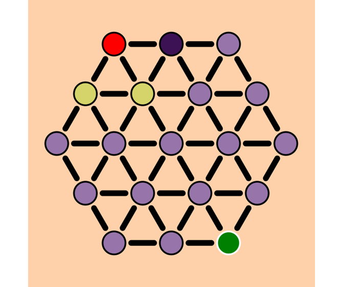
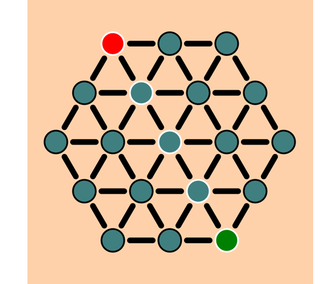
One helpful tool in finding the shortest path is graphs. Graphs are a set of vertices or points connected with edges or arcs. You are allowed to go from one vertex to an other vertex if it is connected with an edge. Below you can see an example of a graph that is layout like a hexagonal grid.
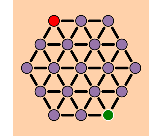
In this image the circles represent the vertices and the lines represent edges.
Path
In the image above two vertices are special. One is colored red, the other is colored green. We would like to know a shortest path from the red vertex to the green vertex.
If we have found a shortest path we will indicate that by highlighting the vertices that we follow along the path.
Algorithm
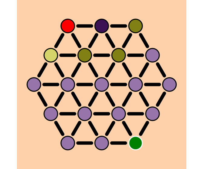
The following series of images will visualize the algorithm we will use to find a path from the red vertex to the green vertex. It starts out by picking a vertex we will examine closer. Because we are at the start we will examine the red vertex.
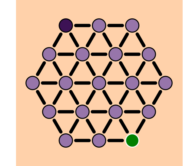
We will look at all the neighbors, i.e. vertices that are connected by an edge, of the vertex we are examining. For the neighbors we now know a path from the red vertex to that particular vertex.
Because we are not at the green vertex yet, we are going to include the neighbors of the vertex we are examining into the frontier. The frontier are the vertices for which we know a path from the red vertex, but we have not examined yet. In other words, they are candidates to examine next.
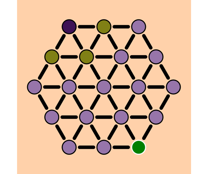
Next we will pick a vertex of the frontier and continue the process. We will have something to say about how to pick a vertex from the frontier shortly. For now we will just pick one.
From this vertex we will examine its neighbors we have not yet visited.
And add those to the frontier.
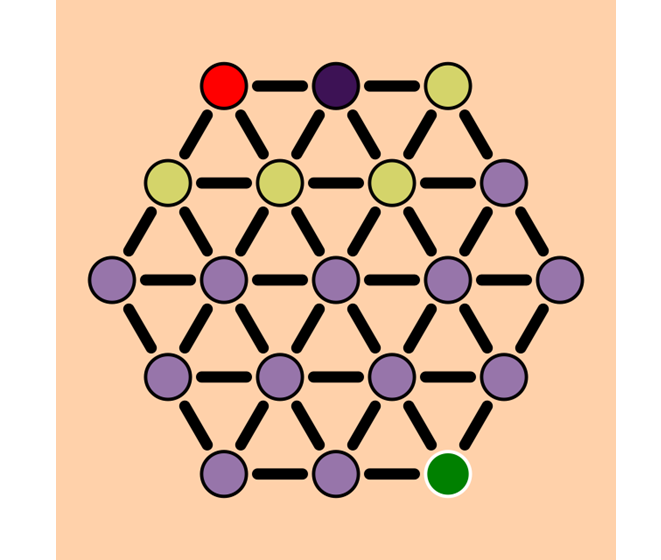
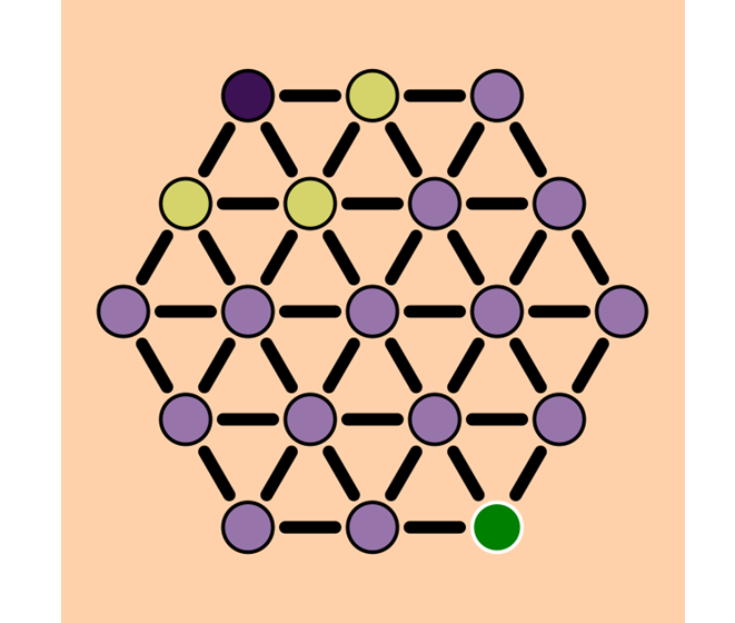
If we continue this process:
We will eventually have visited the green vertex and we know a shortest path from the red vertex to the green vertex.
Pseudocode
We will write down, in pseudocode, an algorithm that can find a shortest path. We assume we are given a graph G, a start vertex start of G and a finish vertex finish of G. We are interested in a shortest path from start to finish and the following algorithm will provide us with one.
for (var v in G.vertices) {
   v.distance = Number.POSITIVE_INFINITY;
}
start.distance = 0;
var frontier = [start];
var visited = [];
while (frontier.length > 0) {
   var current = pickOneOf(frontier);
   for (var neighbour in current.neighbors()) {
       if (neighbour not in visited) {
           neighbour.distance = Math.min(neighbour.distance, current.distance + 1);
           frontier.push(neighbour)
       }
   }
   visited.push(current);
}
We will now annotate the algorithm.
Initialization
We need to initialize some variables that are needed throughout the algorithm.
for (var v in G.vertices) {
   v.distance = Number.POSITIVE_INFINITY;
}
start.distance = 0;
var frontier = [start];
var visited = [];
We first set the distance of all vertices, besides the start vertex to ∞. The distance to the start vertex is set to zero. The frontier will be the collection of vertices for which we know a path but still need to be examined. We initialize it to include the start vertex. Visited will be used to keep track of all vertices that have been examined. Because we still need to examine the start vertex we leave it empty for now.
Loop
We are going to loop until the frontier is empty.
while (frontier.length > 0) {
   // examine a particular vertex in the frontier
}
Because it is possible for the hexagonal grid to reach every vertex from the start vertex, we will end up knowing a shortest path for every vertex. If we are only interested in the shortest path to the finish vertex the condition could be !(finish in visited), i.e. continue as long as we have not visited the finish vertex.
Pick Vertex from Frontier
Within the loop we first pick a vertex from the frontier to examine.
var current = pickOneOf(frontier);This is the heart of the algorithm. Dijkstra, a famous computer scientist, proved that if we pick a vertex of the frontier with the smallest distance, we will end up with a shortest path. Pseudocode for the pickOnOf function could look like:
function pickOneOf(frontier){
   var best = frontier[0];
   for (var candidate in frontier) {
       if (candidate.distance < best.distance) {
           best = candidate;
       }
   }
   return best;
}
Process Neighbors
The current vertex is a vertex with the smallest distance to the start vertex. So we now can determine the distance to the start vertex of the neighbor of the current vertex. We only need to include vertices that we have not visited yet.
for (var neighbour in current.neighbors()) {
   if (neighbour not in visited) {
       /* update neighbour info */
   }
}
Update Neighbour Info
We can now update the information about the neighbour. For instance, if we have found a shorter path we want to update the distance. And we want to add the neighbour to the frontier.
neighbour.distance = Math.min(neighbour.distance, current.distance + 1);
frontier.push(neighbour)
Mark current visited
Finally when we are done examining the current vertex, we add current to the collection of visited.
visited.push(current);Edge Weights
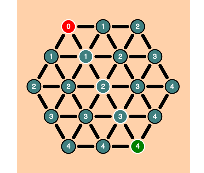
We have included an image where this distance is shown for each vertex.
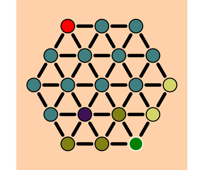
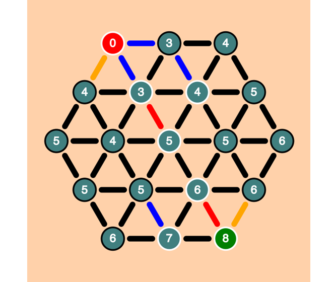
The story gets interesting when we alter the weights of the edges, i.e. the cost to travel over that particular edge. The algorithm needs a small change. When we update the neighbour info we need to use the edge.weight instead of default weight of 1.
In the picture below we have altered the weights of edges, still the algorithm finds a shortest path. The weights of the edges is indicated by the color. A black edge has weight 1, a blue edge has weight 3, an orange edge has weight 5 and a red edge has weight 10.
Live
Seeing an algorithm in action can help you to understand it. You can try this out live in your browser with the following visualization.
Conclusion
We learned that Dijkstra Algorithm can be used to find a shortest path between two vertices of a graph. This in turn can be used to guide enemies over the playing field.
About the author
Daan van Berkel is an enthusiastic software craftsman with a knack for presenting technical details in a clear and concise manner. Driven by the desire for understanding complex matters, Daan is always on the lookout for innovative uses of software.


