NumPy has a number of modules inherited from its predecessor, Numeric. Some of these packages have a SciPy counterpart, which may have fuller functionality.
(For more resources related to this topic, see here.)
Linear algebra
Linear algebra is an important branch of mathematics. The numpy.linalg package contains linear algebra functions. With this module, you can invert matrices, calculate eigenvalues, solve linear equations, and determine determinants, among other things (see http://docs.scipy.org/doc/numpy/reference/routines.linalg.html).
Time for action – inverting matrices
The inverse of a matrix A in linear algebra is the matrix A-1, which, when multiplied with the original matrix, is equal to the identity matrix I. This can be written as follows:
A A-1 = I
The inv() function in the numpy.linalg package can invert an example matrix with the following steps:
Create the example matrix with the mat() function:
A = np.mat("0 1 2;1 0 3;4 -3 8")
print("An", A)
The A matrix appears as follows:
A[[ 0 1 2][ 1 0 3][ 4 -3 8]]
Invert the matrix with the inv() function:
inverse = np.linalg.inv(A)
print("inverse of An", inverse)
If the matrix is singular, or not square, a LinAlgError is raised. If you want, you can check the result manually with a pen and paper. This is left as an exercise for the reader.
Check the result by multiplying the original matrix with the result of the inv() function:
print("Checkn", A * inverse)
The result is the identity matrix, as expected:
Check
[[ 1. 0. 0.]
[ 0. 1. 0.]
[ 0. 0. 1.]]
What just happened?
We calculated the inverse of a matrix with the inv() function of the numpy.linalg package. We checked, with matrix multiplication, whether this is indeed the inverse matrix (see inversion.py):
from __future__ import print_function
import numpy as np
A = np.mat("0 1 2;1 0 3;4 -3 8")
print("An", A)
inverse = np.linalg.inv(A)
print("inverse of An", inverse)
print("Checkn", A * inverse)
Pop quiz – creating a matrix
Q1. Which function can create matrices?
array
create_matrix
mat
vector
Have a go hero – inverting your own matrix
Create your own matrix and invert it. The inverse is only defined for square matrices. The matrix must be square and invertible; otherwise, a LinAlgError exception is raised.
Solving linear systems
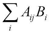
A matrix transforms a vector into another vector in a linear way. This transformation mathematically corresponds to a system of linear equations. The numpy.linalg function solve() solves systems of linear equations of the form Ax = b, where A is a matrix, b can be a one-dimensional or two-dimensional array, and x is an unknown variable. We will see the dot() function in action. This function returns the dot product of two floating-point arrays.
Solve an example of a linear system with the following steps:
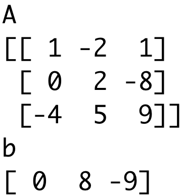
Create A and b:
A = np.mat("1 -2 1;0 2 -8;-4 5 9")
print("An", A)
b = np.array([0, 8, -9])
print("bn", b)
A and b appear as follows:
Solve this linear system with the solve() function:
x = np.linalg.solve(A, b)
print("Solution", x)
The solution of the linear system is as follows:
Solution [ 29. 16. 3.]
Check whether the solution is correct with the dot() function:
print("Checkn", np.dot(A , x))
The result is as expected:
Check[[ 0. 8. -9.]]
What just happened?
We solved a linear system using the solve() function from the NumPy linalg module and checked the solution with the dot() function:
from __future__ import print_function
import numpy as np
A = np.mat("1 -2 1;0 2 -8;-4 5 9")
print("An", A)
b = np.array([0, 8, -9])
print("bn", b)
x = np.linalg.solve(A, b)
print("Solution", x)
print("Checkn", np.dot(A , x))
Time for action – determining eigenvalues and eigenvectors
Let's calculate the eigenvalues of a matrix:
Create a matrix as shown in the following:
A = np.mat("3 -2;1 0")
print("An", A)
The matrix we created looks like the following:
A[[ 3 -2][ 1 0]]
Call the eigvals() function:
print("Eigenvalues", np.linalg.eigvals(A))
The eigenvalues of the matrix are as follows:
Eigenvalues [ 2. 1.]
Determine eigenvalues and eigenvectors with the eig() function. This function returns a tuple, where the first element contains eigenvalues and the second element contains corresponding eigenvectors, arranged column-wise:
eigenvalues, eigenvectors = np.linalg.eig(A)
print("First tuple of eig", eigenvalues)
print("Second tuple of eign", eigenvectors)
The eigenvalues and eigenvectors appear as follows:
First tuple of eig [ 2. 1.]Second tuple of eig[[ 0.89442719 0.70710678][ 0.4472136 0.70710678]]
Check the result with the dot() function by calculating the right and left side of the eigenvalues equation Ax = ax:
for i, eigenvalue in enumerate(eigenvalues):
print("Left", np.dot(A, eigenvectors[:,i]))
print("Right", eigenvalue * eigenvectors[:,i])
print()
The output is as follows:
Left [[ 1.78885438][ 0.89442719]]Right [[ 1.78885438][ 0.89442719]]
What just happened?
We found the eigenvalues and eigenvectors of a matrix with the eigvals() and eig() functions of the numpy.linalg module. We checked the result using the dot() function (see eigenvalues.py):
from __future__ import print_function
import numpy as np
A = np.mat("3 -2;1 0")
print("An", A)
print("Eigenvalues", np.linalg.eigvals(A) )
eigenvalues, eigenvectors = np.linalg.eig(A)
print("First tuple of eig", eigenvalues)
print("Second tuple of eign", eigenvectors)
for i, eigenvalue in enumerate(eigenvalues):
print("Left", np.dot(A, eigenvectors[:,i]))
print("Right", eigenvalue * eigenvectors[:,i])
print()
Singular value decomposition
Singularvaluedecomposition (SVD) is a type of factorization that decomposes a matrix into a product of three matrices. The SVD is a generalization of the previously discussed eigenvalue decomposition. SVD is very useful for algorithms such as the pseudo inverse, which we will discuss in the next section. The svd() function in the numpy.linalg package can perform this decomposition. This function returns three matrices U, ?, and V such that U and V are unitary and ? contains the singular values of the input matrix:
The asterisk denotes the Hermitianconjugate or the conjugatetranspose. The complexconjugate changes the sign of the imaginary part of a complex number and is therefore not relevant for real numbers.
A complex square matrix A is unitary if A*A = AA* = I (the identity matrix). We can interpret SVD as a sequence of three operations—rotation, scaling, and another rotation.
We already transposed matrices in this article. The transpose flips matrices, turning rows into columns, and columns into rows.
Time for action – decomposing a matrix
It's time to decompose a matrix with the SVD using the following steps:
First, create a matrix as shown in the following:
A = np.mat("4 11 14;8 7 -2")
print("An", A)
The matrix we created looks like the following:
A[[ 4 11 14][ 8 7 -2]]
Decompose the matrix with the svd() function:
U, Sigma, V = np.linalg.svd(A, full_matrices=False)
print("U")
print(U)
print("Sigma")
print(Sigma)
print("V")
print(V)
Because of the full_matrices=False specification, NumPy performs a reduced SVD decomposition, which is faster to compute. The result is a tuple containing the two unitary matrices U and V on the left and right, respectively, and the singular values of the middle matrix:
U
[[-0.9486833 -0.31622777]
[-0.31622777 0.9486833 ]]
Sigma
[ 18.97366596 9.48683298]
V
[[-0.33333333 -0.66666667 -0.66666667]
[ 0.66666667 0.33333333 -0.66666667]]
We do not actually have the middle matrix—we only have the diagonal values. The other values are all 0. Form the middle matrix with the diag() function. Multiply the three matrices as follows:
print("Productn", U * np.diag(Sigma) * V)
The product of the three matrices is equal to the matrix we created in the first step:
Product
[[ 4. 11. 14.]
[ 8. 7. -2.]]
What just happened?
We decomposed a matrix and checked the result by matrix multiplication. We used the svd() function from the NumPy linalg module (see decomposition.py):
from __future__ import print_function
import numpy as np
A = np.mat("4 11 14;8 7 -2")
print("An", A)
U, Sigma, V = np.linalg.svd(A, full_matrices=False)
print("U")
print(U)
print("Sigma")
print(Sigma)
print("V")
print(V)
print("Productn", U * np.diag(Sigma) * V)
Pseudo inverse
The Moore-Penrose pseudo inverse of a matrix can be computed with the pinv() function of the numpy.linalg module (see http://en.wikipedia.org/wiki/Moore%E2%80%93Penrose_pseudoinverse). The pseudo inverse is calculated using the SVD (see previous example). The inv() function only accepts square matrices; the pinv() function does not have this restriction and is therefore considered a generalization of the inverse.
Time for action – computing the pseudo inverse of a matrix
Let's compute the pseudo inverse of a matrix:
First, create a matrix:
A = np.mat("4 11 14;8 7 -2")
print("An", A)
The matrix we created looks like the following:
A[[ 4 11 14][ 8 7 -2]]
Calculate the pseudo inverse matrix with the pinv() function:
We computed the pseudo inverse of a matrix with the pinv() function of the numpy.linalg module. The check by matrix multiplication resulted in a matrix that is approximately an identity matrix (see pseudoinversion.py):
from __future__ import print_function
import numpy as np
A = np.mat("4 11 14;8 7 -2")
print("An", A)
pseudoinv = np.linalg.pinv(A)
print("Pseudo inversen", pseudoinv)
print("Check", A * pseudoinv)
Determinants
The determinant is a value associated with a square matrix. It is used throughout mathematics; for more details, please refer to http://en.wikipedia.org/wiki/Determinant. For a n x n real value matrix, the determinant corresponds to the scaling a n-dimensional volume undergoes when transformed by the matrix. The positive sign of the determinant means the volume preserves its orientation (clockwise or anticlockwise), while a negative sign means reversed orientation. The numpy.linalg module has a det() function that returns the determinant of a matrix.
Time for action – calculating the determinant of a matrix
To calculate the determinant of a matrix, follow these steps:
Unlock access to the largest independent learning library in Tech for FREE!
Get unlimited access to 7500+ expert-authored eBooks and video courses covering every tech area you can think of.
Renews at $19.99/month. Cancel anytime
Create the matrix:
A = np.mat("3 4;5 6")
print("An", A)
The matrix we created appears as follows:
A[[ 3. 4.][ 5. 6.]]
Compute the determinant with the det() function:
print("Determinant", np.linalg.det(A))
The determinant appears as follows:
Determinant -2.0
What just happened?
We calculated the determinant of a matrix with the det() function from the numpy.linalg module (see determinant.py):
from __future__ import print_function
import numpy as np
A = np.mat("3 4;5 6")
print("An", A)
print("Determinant", np.linalg.det(A))
Fast Fourier transform
The FastFouriertransform (FFT) is an efficient algorithm to calculate the discreteFouriertransform (DFT).
The Fourier series represents a signal as a sum of sine and cosine terms.
FFT improves on more naïve algorithms and is of order O(N log N). DFT has applications in signal processing, image processing, solving partial differential equations, and more. NumPy has a module called fft that offers FFT functionality. Many functions in this module are paired; for those functions, another function does the inverse operation. For instance, the fft() and ifft() function form such a pair.
Time for action – calculating the Fourier transform
First, we will create a signal to transform. Calculate the Fourier transform with the following steps:
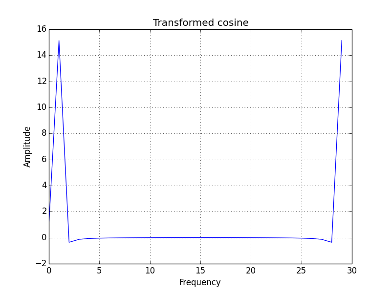
Create a cosine wave with 30 points as follows:
x = np.linspace(0, 2 * np.pi, 30)
wave = np.cos(x)
Transform the cosine wave with the fft() function:
transformed = np.fft.fft(wave)
Apply the inverse transform with the ifft() function. It should approximately return the original signal. Check with the following line:
The following resulting diagram shows the FFT result:
What just happened?
We applied the fft() function to a cosine wave. After applying the ifft() function, we got our signal back (see fourier.py):
from __future__ import print_function
import numpy as np
import matplotlib.pyplot as plt
x = np.linspace(0, 2 * np.pi, 30)
wave = np.cos(x)
transformed = np.fft.fft(wave)
print(np.all(np.abs(np.fft.ifft(transformed) - wave) < 10 ** -9))
plt.plot(transformed)
plt.title('Transformed cosine')
plt.xlabel('Frequency')
plt.ylabel('Amplitude')
plt.grid()
plt.show()
Shifting
The fftshift() function of the numpy.linalg module shifts zero-frequency components to the center of a spectrum. The zero-frequency component corresponds to the mean of the signal. The ifftshift() function reverses this operation.
Time for action – shifting frequencies
We will create a signal, transform it, and then shift the signal. Shift the frequencies with the following steps:
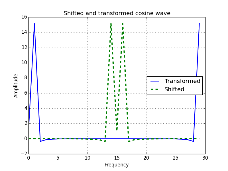
Create a cosine wave with 30 points:
x = np.linspace(0, 2 * np.pi, 30)
wave = np.cos(x)
Transform the cosine wave with the fft() function:
transformed = np.fft.fft(wave)
Shift the signal with the fftshift() function:
shifted = np.fft.fftshift(transformed)
Reverse the shift with the ifftshift() function. This should undo the shift. Check with the following code snippet:
Random numbers are used in Monte Carlo methods, stochastic calculus, and more. Real random numbers are hard to generate, so, in practice, we use pseudorandomnumbers, which are random enough for most intents and purposes, except for some very special cases. These numbers appear random, but if you analyze them more closely, you will realize that they follow a certain pattern. The random numbers-related functions are in the NumPy random module. The core random number generator is based on the MersenneTwisteralgorithm—a standard and well-known algorithm (see https://en.wikipedia.org/wiki/Mersenne_Twister). We can generate random numbers from discrete or continuous distributions. The distribution functions have an optional size parameter, which tells NumPy how many numbers to generate. You can specify either an integer or a tuple as size. This will result in an array filled with random numbers of appropriate shape. Discrete distributions include the geometric, hypergeometric, and binomial distributions.
Imagine a 17th century gambling house where you can bet on flipping pieces of eight. Nine coins are flipped. If less than five are heads, then you lose one piece of eight, otherwise you win one. Let's simulate this, starting with 1,000 coins in our possession. Use the binomial() function from the random module for that purpose.
To understand the binomial() function, look at the following section:
Initialize an array, which represents the cash balance, to zeros. Call the binomial() function with a size of 10000. This represents 10,000 coin flips in our casino:
Go through the outcomes of the coin flips and update the cash array. Print the minimum and maximum of the outcome, just to make sure we don't have any strange outliers:
for i in range(1, len(cash)):
if outcome[i] < 5:
cash[i] = cash[i - 1] - 1
elif outcome[i] < 10:
cash[i] = cash[i - 1] + 1
else:
raise AssertionError("Unexpected outcome " + outcome)
print(outcome.min(), outcome.max())
As expected, the values are between 0 and 9. In the following diagram, you can see the cash balance performing a random walk:
What just happened?
We did a random walk experiment using the binomial() function from the NumPy random module (see headortail.py):
from __future__ import print_function
import numpy as np
import matplotlib.pyplot as plt
cash = np.zeros(10000)
cash[0] = 1000
np.random.seed(73)
outcome = np.random.binomial(9, 0.5, size=len(cash))
for i in range(1, len(cash)):
if outcome[i] < 5:
cash[i] = cash[i - 1] - 1
elif outcome[i] < 10:
cash[i] = cash[i - 1] + 1
else:
raise AssertionError("Unexpected outcome " + outcome)
print(outcome.min(), outcome.max())
plt.plot(np.arange(len(cash)), cash)
plt.title('Binomial simulation')
plt.xlabel('# Bets')
plt.ylabel('Cash')
plt.grid()
plt.show()
Hypergeometric distribution
The hypergeometricdistribution models a jar with two types of objects in it. The model tells us how many objects of one type we can get if we take a specified number of items out of the jar without replacing them (see https://en.wikipedia.org/wiki/Hypergeometric_distribution). The NumPy random module has a hypergeometric() function that simulates this situation.
Time for action – simulating a game show
Imagine a game show where every time the contestants answer a question correctly, they get to pull three balls from a jar and then put them back. Now, there is a catch, one ball in the jar is bad. Every time it is pulled out, the contestants lose six points. If, however, they manage to get out 3 of the 25 normal balls, they get one point. So, what is going to happen if we have 100 questions in total? Look at the following section for the solution:
Initialize the outcome of the game with the hypergeometric() function. The first parameter of this function is the number of ways to make a good selection, the second parameter is the number of ways to make a bad selection, and the third parameter is the number of items sampled:
Set the scores based on the outcomes from the previous step:
for i in range(len(points)):
if outcomes[i] == 3:
points[i] = points[i - 1] + 1
elif outcomes[i] == 2:
points[i] = points[i - 1] - 6
else:
print(outcomes[i])
The following diagram shows how the scoring evolved:
What just happened?
We simulated a game show using the hypergeometric() function from the NumPy random module. The game scoring depends on how many good and how many bad balls the contestants pulled out of a jar in each session (see urn.py):
from __future__ import print_function
import numpy as np
import matplotlib.pyplot as plt
points = np.zeros(100)
np.random.seed(16)
outcomes = np.random.hypergeometric(25, 1, 3, size=len(points))
for i in range(len(points)):
if outcomes[i] == 3:
points[i] = points[i - 1] + 1
elif outcomes[i] == 2:
points[i] = points[i - 1] - 6
else:
print(outcomes[i])
plt.plot(np.arange(len(points)), points)
plt.title('Game show simulation')
plt.xlabel('# Rounds')
plt.ylabel('Score')
plt.grid()
plt.show()
Continuous distributions
We usually model continuous distributions with probability density functions (PDF). The probability that a value is in a certain interval is determined by integration of the PDF (see https://www.khanacademy.org/math/probability/random-variables-topic/random_variables_prob_dist/v/probability-density-functions). The NumPy random module has functions that represent continuous distributions—beta(), chisquare(), exponential(), f(), gamma(), gumbel(), laplace(), lognormal(), logistic(), multivariate_normal(), noncentral_chisquare(), noncentral_f(), normal(), and others.
In the following diagram, we see the familiar bell curve:
What just happened?
We visualized the normal distribution using the normal() function from the random NumPy module. We did this by drawing the bell curve and a histogram of randomly generated values (see normaldist.py):
A lognormal distribution is a distribution of a random variable whose natural logarithm is normally distributed. The lognormal() function of the random NumPy module models this distribution.
Time for action – drawing the lognormal distribution
Let's visualize the lognormal distribution and its PDF with a histogram:
Generate random numbers using the normal() function from the random NumPy module:
The fit of the histogram and theoretical PDF is excellent, as you can see in the following diagram:
What just happened?
We visualized the lognormal distribution using the lognormal() function from the random NumPy module. We did this by drawing the curve of the theoretical PDF and a histogram of randomly generated values (see lognormaldist.py):
Bootstrapping is a method used to estimate variance, accuracy, and other metrics of sample estimates, such as the arithmetic mean. The simplest bootstrapping procedure consists of the following steps:
Generate a large number of samples from the original data sample having the same size N. You can think of the original data as a jar containing numbers. We create the new samples by N times randomly picking a number from the jar. Each time we return the number into the jar, so a number can occur multiple times in a generated sample.
With the new samples, we calculate the statistical estimate under investigation for each sample (for example, the arithmetic mean). This gives us a sample of possible values for the estimator.
Time for action – sampling with numpy.random.choice()
We will use the numpy.random.choice() function to perform bootstrapping.
Start the IPython or Python shell and import NumPy:
$ ipythonIn [1]: import numpy as np
Generate a data sample following the normal distribution:
In [2]: N = 500In [3]: np.random.seed(52)In [4]: data = np.random.normal(size=N)
Calculate the mean of the data:
In [5]: data.mean()Out[5]: 0.07253250605445645
Generate 100 samples from the original data and calculate their means (of course, more samples may lead to a more accurate result):
In [6]: bootstrapped = np.random.choice(data, size=(N, 100))In [7]: means = bootstrapped.mean(axis=0)In [8]: means.shapeOut[8]: (100,)
Calculate the mean, variance, and standard deviation of the arithmetic means we obtained:
In [9]: means.mean()Out[9]: 0.067866373318115278In [10]: means.var()Out[10]: 0.001762807104774598In [11]: means.std()Out[11]: 0.041985796464692651
If we are assuming a normal distribution for the means, it may be relevant to know the z-score, which is defined as follows:
In [12]: (data.mean() - means.mean())/means.std()Out[12]: 0.11113598238549766
From the z-score value, we get an idea of how probable the actual mean is.
What just happened?
We bootstrapped a data sample by generating samples and calculating the means of each sample. Then we computed the mean, standard deviation, variance, and z-score of the means. We used the numpy.random.choice() function for bootstrapping.
Summary
You learned a lot in this article about NumPy modules. We covered linear algebra, the Fast Fourier transform, continuous and discrete distributions, and random numbers.

 United States
 Great Britain
 India
India
 Germany
 France
 Canada
 Russia
 Spain
Spain
 Brazil
 Australia
 Singapore
 Canary Islands
 Hungary
 Ukraine
 Luxembourg
 Estonia
 Lithuania
 South Korea
 Turkey
 Switzerland
 Colombia
 Taiwan
 Chile
Chile
 Norway
 Ecuador
 Indonesia
 New Zealand
 Cyprus
 Denmark
 Finland
 Poland
 Malta
Malta
 Czechia
 Austria
 Sweden
 Italy
Italy
 Egypt
Egypt
 Belgium
 Portugal
 Slovenia
 Ireland
 Romania
 Greece
 Argentina
 Netherlands
 Bulgaria
 Latvia
 South Africa
 Malaysia
 Japan
Japan
 Slovakia
 Philippines
 Mexico
 Thailand