In this article by Francisco J. Blanco-Silva, author of the book Mastering SciPy, you will learn about image editing and the purpose of editing is the alteration of digital images, usually to perform improvement of its properties or to turn them into an intermediate step for further processing.

Let’s examine different examples of editing:

• Transformations of the domain
• Intensity adjustment
• Image restoration

(For more resources related to this topic, see here.)

Transformations of the domain

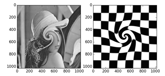
In this setting, we address transformations to images by first changing the location of pixels, rotations, compressions, stretching, swirls, cropping, perspective control, and so on. Once the transformation to the pixels in the domain of the original is performed, we observe the size of the output. If there are more pixels in this image than in the original, the extra locations are filled with numerical values obtained by interpolating the given data. We do have some control over the kind of interpolation performed, of course. To better illustrate these techniques, we will pair an actual image (say, Lena) with a representation of its domain as a checkerboard:

In [1]: import numpy as np, matplotlib.pyplot as plt

In [2]: from scipy.misc import lena; 

   ...: from skimage.data import checkerboard

In [3]: image = lena().astype('float')

   ...: domain = checkerboard()

In [4]: print image.shape, domain.shape

Out[4]: (512, 512) (200, 200)

Rescale and resize

Before we proceed with the pairing of image and domain, we have to make sure that they both have the same size. One quick fix is to rescale both objects, or simply resize one of the images to match the size of the other. Let’s go with the first choice, so that we can illustrate the usage of the two functions available for this task in the module skimage.transform to resize and rescale:

In [5]: from skimage.transform import rescale, resize

In [6]: domain = rescale(domain, scale=1024./200); 

   ...: image = resize(image, output_shape=(1024, 1024), order=3)

Observe how, in the resizing operation, we requested a bicubic interpolation.

Swirl

To perform a swirl, we call the function swirl from the module skimage.transform:

In all the examples of this section, we will present the results visually after performing the requested computations. In all cases, the syntax of the call to offer the images is the same. For a given operation mapping, we issue the command display (mapping, image, and domain) where the routine display is defined as follows:

def display(mapping, image, domain):

   plt.figure()

   plt.subplot(121)

 plt.imshow(mapping(image))

   plt.gray()

   plt.subplot(122)

   plt.imshow(mapping(domain))

   plt.show()

For the sake of brevity, we will not include this command in the following code, but assume it is called every time:

In [7]: from skimage.transform import swirl

In [8]: mapping = lambda img: swirl(img, strength=6,

   ...:                                 radius=512)

Geometric transformations

A simple rotation around any location (no matter whether inside or outside the domain of the image) can be achieved with the function rotate from either module scipy.ndimage or skimage.transform. They are basically the same under the hood, but the syntax of the function in the scikit-image toolkit is more user-friendly:

In [10]: from skimage.transform import rotate

In [11]: mapping = lambda img: rotate(img, angle=30, resize=True,

   ....:                             center=None)

This gives a counter-clockwise rotation of 30 degrees (angle=30) around the center of the image (center=None). The size of the output image is expanded to guarantee that all the original pixels are present in the output (resize=True):

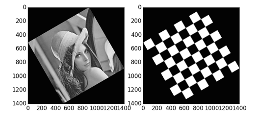
Rotations are a special case of what we call an affine transformation—a combination of rotation with scales (one for each dimension), shear, and translation. Affine transformations are in turn a special case of a homography (a projective transformation). Rather than learning a different set of functions, one for each kind of geometric transformation, the library skimage.transform allows a very comfortable setting. There is a common function (warp) that gets called with the requested geometric transformation and performs the computations. Each suitable geometric transformation is previously initialized with an appropriate python class. For example, to perform an affine transformation with a counter-clockwise rotation angle of 30 degrees about the point with coordinates (512, -2048), and scale factors of 2 and 3 units, respectively for the x and y coordinates, we issue the following command:

In [13]: from skimage.transform import warp, AffineTransform

In [14]: operation = AffineTransform(scale=(2,3), rotation=np.pi/6, 

   ....:                             translation = (512, -2048))

In [15]: mapping = lambda img: warp(img, operation)

Observe how all the lines in the transformed checkerboard are either parallel or perpendicular—affine transformations preserve angles.

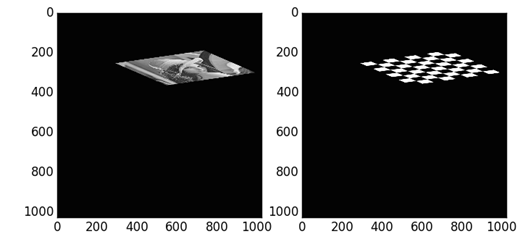
The following illustrates the effect of a homography:

In [17]: from skimage.transform import ProjectiveTransform

In [18]: generator = np.matrix('1,0,10; 0,1,20; -0.0007,0.0005,1'); 

   ....: homography = ProjectiveTransform(matrix=generator); 

   ....: mapping = lambda img: warp(img, homography)

Observe how, unlike in the case of an affine transformation, the lines cease to be all parallel or perpendicular. All vertical lines are now incident at a point at infinity. All horizontal lines are also incident at a different point at infinity.

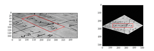
The real usefulness of homographies arises, for example, when we need to perform perspective control. For instance, the image skimage.data.text is clearly slanted. By choosing the four corners of what we believe is a perfect rectangle (we estimate such a rectangle by visual inspection), we can compute a homography that transforms the given image into one that is devoid of any perspective. The Python classes representing geometric transformations allow us to perform this estimation very easily, as the following example shows:

In [20]: from skimage.data import text

In [21]: text().shape

Out[21]: (172, 448)

In [22]: source = np.array(((155, 15), (65, 40),

   ....:                   (260, 130), (360, 95),

   ....:                   (155, 15)))

In [23]: mapping = ProjectiveTransform()

Let’s estimate the homography that transforms the given set of points into a perfect rectangle of the size 48 x 256 centered in an output image of size 512 x 512. The choice of size of the output image is determined by the length of the diagonal of the original image (about 479 pixels). This way, after the homography is computed, the output is likely to contain all the pixels from the original.

Observe that we have included one of vertices in the source, twice. This is not strictly necessary for the following computations, but will make the visualization of rectangles much easier to code. We use the same trick for the target rectangle.

In [24]: target = np.array(((256-128, 256-24), (256-128, 256+24),

   ....:                   (256+128, 256+24), (256+128, 256-24),

   ....:                   (256-128, 256-24)))

In [25]: mapping.estimate(target, source)

Out[25]: True

In [26]: plt.figure(); 

   ....: plt.subplot(121); 

   ....: plt.imshow(text()); 

   ....: plt.gray(); 

   ....: plt.plot(source[:,0], source[:,1],'-', lw=1, color='red'); 

   ....: plt.xlim(0, 448); 

   ....: plt.ylim(172, 0); 

   ....: plt.subplot(122); 

   ....: plt.imshow(warp(text(), mapping,output_shape=(512, 512))); 

   ....: plt.plot(target[:,0], target[:,1],'-', lw=1, color='red'); 

   ....: plt.xlim(0, 512); 

   ....: plt.ylim(512, 0); 

   ....: plt.show()

Other more involved geometric operations are needed, for example, to fix vignetting and some of the other kinds of distortions produced by photographic lenses. Traditionally, once we acquire an image, we assume that all these distortions are present. By knowing the technical specifications of the equipment used to take the photographs, we can automatically rectify these defects. With this purpose in mind, in the SciPy stack, we have access to the lensfun library (http://lensfun.sourceforge.net/) through the package lensfunpy (https://pypi.python.org/pypi/lensfunpy).

For examples of usage and documentation, an excellent resource is the API reference of lensfunpy at http://pythonhosted.org/lensfunpy/api/.

Intensity adjustment

In this category, we have operations that only modify the intensity of an image obeying a global formula. All these operations can therefore be easily coded by using purely NumPy operations, by creating vectorized functions adapting the requested formulas.

The applications of these operations can be explained in terms of exposure in black and white photography, for example. For this reason, all the examples in this section are applied on gray-scale images.

We have mainly three approaches to enhancing images by working on its intensity:

• Histogram equalizations
• Intensity clipping/resizing
• Contrast adjustment

Histogram equalization

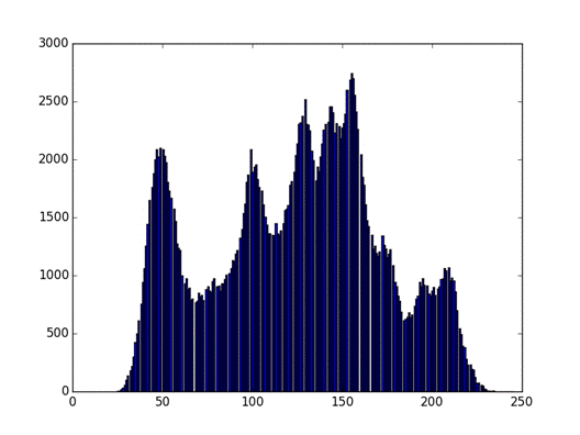
The starting point in this setting is always the concept of intensity histogram (or more precisely, the histogram of pixel intensity values)—a function that indicates the number of pixels in an image at each different intensity value found in that image.

For instance, for the original version of Lena, we could issue the following command:

In [27]: plt.figure(); 

   ....: plt.hist(lena().flatten(), 256); 

   ....: plt.show()

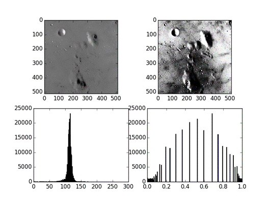
The operations of histogram equalization improve the contrast of images by modifying the histogram in a way that most of the relevant intensities have the same impact. We can accomplish this enhancement by calling, from the module skimage.exposure, any of the functions equalize_hist (pure histogram equalization) or equalize_adaphist (contrast limited adaptive histogram equalization (CLAHE)).

Note the obvious improvement after the application of the histogram equalization of the image skimage.data.moon.

In the following examples, we include the corresponding histogram below all relevant images for comparison. A suitable code to perform this visualization could be as follows:

def display(image, transform, bins):

   target = transform(image)

   plt.figure()

   plt.subplot(221)

   plt.imshow(image)

   plt.gray()

   plt.subplot(222)

   plt.imshow(target)

   plt.subplot(223)

   plt.hist(image.flatten(), bins)

   plt.subplot(224)

   plt.hist(target.flatten(), bins)

   plt.show()

In [28]: from skimage.exposure import equalize_hist; 

   ....: from skimage.data import moon

In [29]: display(moon(), equalize_hist, 256)

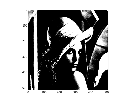
Intensity clipping/resizing

A peak at the histogram indicates the presence of a particular intensity that is remarkably more predominant than its neighboring ones. If we desire to isolate intensities around a peak, we can do so using purely NumPy masking/clipping operations on the original image. If storing the result is not needed, we can request a quick visualization of the result by employing the command clim in the library matplotlib.pyplot. For instance, to isolate intensities around the highest peak of Lena (roughly, these are between 150 and 160), we could issue the following command:

In [30]: plt.figure(); 

   ....: plt.imshow(lena()); 

   ....: plt.clim(vmin=150, vmax=160); 

   ....: plt.show()

Note how this operation, in spite of having reduced the representative range of intensities from 256 to 10, offers us a new image that keeps sufficient information to recreate the original one. Naturally, we can regard this operation also as a lossy compression method.

Contrast enhancement

An obvious drawback of clipping intensities is the loss of perceived lightness contrast. To overcome this loss, it is preferable to employ formulas that do not reduce the size of the range. Among the many available formulas conforming to this mathematical property, the most successful ones are those that replicate an optical property of the acquisition method. We explore the following three cases:

• Gamma correction: Human vision follows a power function, with greater sensitivity to relative differences between darker tones than between lighter ones. Each original image, as captured by the acquisition device, might allocate too many bits or too much bandwidth to highlight that humans cannot actually differentiate. Similarly, too few bits/bandwidth could be allocated to the darker areas of the image. By manipulation of this power function, we are capable of addressing the correct amount of bits and bandwidth.
• Sigmoid correction: Independently of the amount of bits and bandwidth, it is often desirable to maintain the perceived lightness contrast. Sigmoidal remapping functions were then designed based on empirical contrast enhancement model developed from the results of psychophysical adjustment experiments.
• Logarithmic correction: This is a purely mathematical process designed to spread the range of naturally low-contrast images by transforming to a logarithmic range.

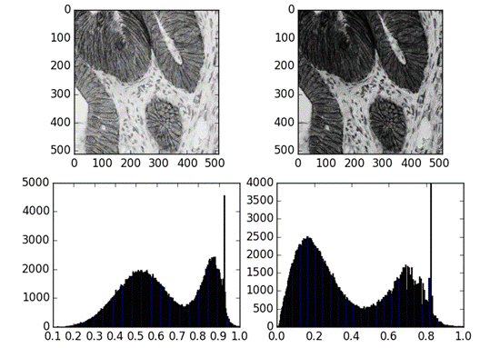
To perform gamma correction on images, we could employ the function adjust_gamma in the module skimage.exposure. The equivalent mathematical operation is the power-law relationship output = gain * input^gamma. Observe the great improvement in definition of the brighter areas of a stained micrograph of colonic glands, when we choose the exponent gamma=2.5 and no gain (gain=1.0):

In [31]: from skimage.exposure import adjust_gamma; 

   ....: from skimage.color import rgb2gray; 

   ....: from skimage.data import immunohistochemistry

In [32]: image = rgb2gray(immunohistochemistry())

In [33]: correction = lambda img: adjust_gamma(img, gamma=2.5,

   ....:                                       gain=1.)

Note the huge improvement in contrast in the lower right section of the micrograph, allowing a better description and differentiation of the observed objects:

Immunohistochemical staining with hematoxylin counterstaining. This image was acquired at the Center for Microscopy And Molecular Imaging (CMMI).

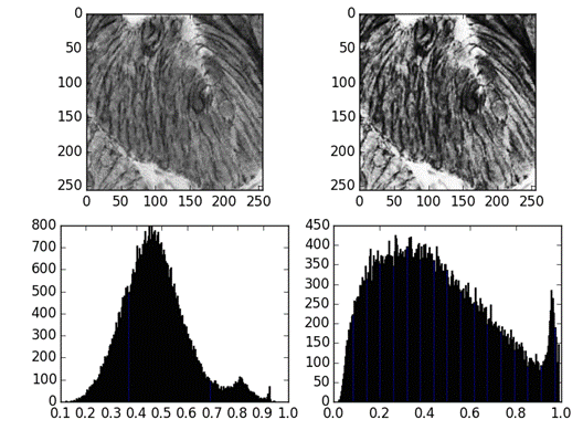
To perform sigmoid correction with given gain and cutoff coefficients, according to the formula output = 1/(1 + exp*(gain*(cutoff – input))), we employ the function adjust_sigmoid in skimage.exposure. For example, with gain=10.0 and cutoff=0.5 (the default values), we obtain the following enhancement:

In [35]: from skimage.exposure import adjust_sigmoid

In [36]: display(image[:256, :256], adjust_sigmoid, 256)

Note the improvement in the definition of the walls of cells in the enhanced image:

We have already explored logarithmic correction in the previous section, when enhancing the visualization of the frequency of an image. This is equivalent to applying a vectorized version of np.log1p to the intensities. The corresponding function in the scikit-image toolkit is adjust_log in the sub module exposure.

Image restoration

In this category of image editing, the purpose is to repair the damage produced by post or preprocessing of the image, or even the removal of distortion produced by the acquisition device. We explore two classic situations:

• Noise reduction
• Sharpening and blurring

Noise reduction

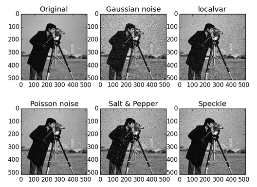
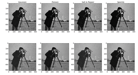
In mathematical imaging, noise is by definition a random variation of the intensity (or the color) produced by the acquisition device. Among all the possible types of noise, we acknowledge four key cases:

• Gaussian noise: We add to each pixel a value obtained from a random variable with normal distribution and a fixed mean. We usually allow the same variance on each pixel of the image, but it is feasible to change the variance depending on the location.
• Poisson noise: To each pixel, we add a value obtained from a random variable with Poisson distribution.
• Salt and pepper: This is a replacement noise, where some pixels are substituted by zeros (black or pepper), and some pixels are substituted by ones (white or salt).
• Speckle: This is a multiplicative kind of noise, where each pixel gets modified by the formula output = input + n * input. The value of the modifier n is a value obtained from a random variable with uniform distribution of fixed mean and variance.

To emulate all these kinds of noise, we employ the utility random_noise from the module skimage.util. Let’s illustrate the possibilities in a common image:

In [37]: from skimage.data import camera; 

   ....: from skimage.util import random_noise

In [38]: gaussian_noise = random_noise(camera(), 'gaussian',

   ....:                               var=0.025); 

   ....: poisson_noise = random_noise(camera(), 'poisson'); 

   ....: saltpepper_noise = random_noise(camera(), 's&p',

   ....:                                salt_vs_pepper=0.45); 

   ....: speckle_noise = random_noise(camera(), 'speckle', var=0.02)

In [39]: variance_generator = lambda i,j: 0.25*(i+j)/1022. + 0.001; 

   ....: variances = np.fromfunction(variance_generator,(512,512)); 

   ....: lclvr_noise = random_noise(camera(), 'localvar',

   ....:                           local_vars=variances)

In the last example, we have created a function that assigns a variance between 0.001 and 0.026 depending on the distance to the upper corner of an image. When we visualize the corresponding noisy version of skimage.data.camera, we see that the level of degradation gets stronger as we get closer to the lower right corner of the picture.

The following is an example of visualization of the corresponding noisy images:

The purpose of noise reduction is to remove as much of this unwanted signal, so we obtain an image as close to the original as possible. The trick, of course, is to do so without any previous knowledge of the properties of the noise.

The most basic methods of denoising are the application of either a Gaussian or a median filter. We explored them both in the previous section. The former was presented as a smoothing filter (gaussian_filter), and the latter was discussed when we explored statistical filters (median_filter). They both offer decent noise removal, but they introduce unwanted artifacts as well. For example, the Gaussian filter does not preserve edges in images. The application of any of these methods is also not recommended if preserving texture information is needed.

We have a few more advanced methods in the module skimage.restoration, able to tailor denoising to images with specific properties:

• denoise_bilateral: This is the bilateral filter. It is useful when preserving edges is important.
• denoise_tv_bregman, denoise_tv_chambolle: We will use this if we require a denoised image with small total variation.
• nl_means_denoising: The so-called non-local means denoising. This method ensures the best results to denoise areas of the image presenting texture.
• wiener, unsupervised_wiener: This is the Wiener-Hunt deconvolution. It is useful when we have knowledge of the point-spread function at acquisition time.

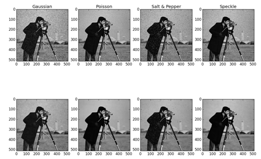
Let’s show you, by example, the performance of one of these methods on some of the noisy images we computed earlier:

In [40]: from skimage.restoration import nl_means_denoising as dnoise

In [41]: images = [gaussian_noise, poisson_noise,

   ....:           saltpepper_noise, speckle_noise]; 

   ....: names = ['Gaussian', 'Poisson', 'Salt & Pepper', 'Speckle']

In [42]: plt.figure()

Out[42]: <matplotlib.figure.Figure at 0x118301490>

In [43]: for index, image in enumerate(images):

   ....:     output = dnoise(image, patch_size=5, patch_distance=7)

   ....:     plt.subplot(2, 4, index+1)

   ....:    plt.imshow(image)

   ....:     plt.gray()

   ....:     plt.title(names[index])

   ....:     plt.subplot(2, 4, index+5)

   ....:     plt.imshow(output)

   ....:

In [44]: plt.show()

Under each noisy image, we have presented the corresponding result after employing, by nonlocal means, denoising:

It is also possible to perform denoising by thresholding coefficient, provided we represent images with a transform. For example, to do a soft thresholding, employing Biorthonormal 2.8 wavelets; we will use the package PyWavelets:

In [45]: import pywt

In [46]: def dnoise(image, wavelet, noise_var):

   ....:     levels = int(np.floor(np.log2(image.shape[0])))

   ....:     coeffs = pywt.wavedec2(image, wavelet, level=levels)

   ....:     value = noise_var * np.sqrt(2 * np.log2(image.size))

   ....:     threshold = lambda x: pywt.thresholding.soft(x, value)

   ....:     coeffs = map(threshold, coeffs)

   ....:     return pywt.waverec2(coeffs, wavelet)

   ....:

In [47]: plt.figure()

Out[47]: <matplotlib.figure.Figure at 0x10e5ed790>

In [48]: for index, image in enumerate(images):

   ....:     output = dnoise(image, pywt.Wavelet('bior2.8'),

   ....:                     noise_var=0.02)

   ....:     plt.subplot(2, 4, index+1)

   ....:     plt.imshow(image)

   ....:     plt.gray()

   ....:     plt.title(names[index])

   ....:     plt.subplot(2, 4, index+5)

   ....:     plt.imshow(output)

   ....:

In [49]: plt.show()

Observe that the results are of comparable quality to those obtained with the previous method:

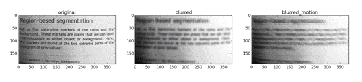
Sharpening and blurring

There are many situations that produce blurred images:

• Incorrect focus at acquisition
• Movement of the imaging system
• The point-spread function of the imaging device (like in electron microscopy)
• Graphic-art effects

For blurring images, we could replicate the effect of a point-spread function by performing convolution of the image with the corresponding kernel. The Gaussian filter that we used for denoising performs blurring in this fashion. In the general case, convolution with a given kernel can be done with the routine convolve from the module scipy.ndimage. For instance, for a constant kernel supported on a 10 x 10 square, we could do as follows:

In [50]: from scipy.ndimage import convolve; 

   ....: from skimage.data import page

In [51]: kernel = np.ones((10, 10))/100.; 

   ....: blurred = convolve(page(), kernel)

To emulate the blurring produced by movement too, we could convolve with a kernel as created here:

In [52]: from skimage.draw import polygon

In [53]: x_coords = np.array([14, 14, 24, 26, 24, 18, 18]); 

   ....: y_coords = np.array([ 2, 18, 26, 24, 22, 18, 2]); 

   ....: kernel_2 = np.zeros((32, 32)); 

   ....: kernel_2[polygon(x_coords, y_coords)]= 1.; 

   ....: kernel_2 /= kernel_2.sum()

In [54]: blurred_motion = convolve(page(), kernel_2)

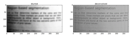
In order to reverse the effects of convolution when we have knowledge of the degradation process, we perform deconvolution. For example, if we have knowledge of the point-spread function, in the module skimage.restoration we have implementations of the Wiener filter (wiener), the unsupervised Wiener filter (unsupervised_wiener), and Lucy-Richardson deconvolution (richardson_lucy).

We perform deconvolution on blurred images by applying a Wiener filter. Note the huge improvement in readability of the text:

In [55]: from skimage.restoration import wiener

In [56]: deconv = wiener(blurred, kernel, balance=0.025, clip=False)

Summary

In this article, we have seen how the SciPy stack helps us solve many problems in mathematical imaging, from the effective representation of digital images, to modifying, restoring, or analyzing them. Although certainly exhaustive, this article scratches but the surface of this challenging field of engineering.

Resources for Article:

---

Further resources on this subject:

• Symbolizers [article]
• Machine Learning [article]
• Analyzing a Complex Dataset [article]

---