In this article by Pratap Dangeti, the author of the book Statistics for Machine Learning, we will take a look at ridge regression and lasso regression in machine learning.

(For more resources related to this topic, see here.)

Ridge regression and lasso regression

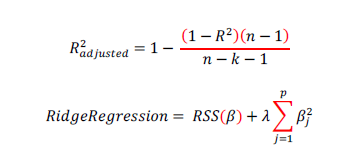
In linear regression only residual sum of squares (RSS) are minimized, whereas in ridge and lasso regression, penalty applied (also known as shrinkage penalty) on coefficient values to regularize the coefficients with the tuning parameter λ.

When λ=0 penalty has no impact, ridge/lasso produces the same result as linear regression, whereas λ => ∞ will bring coefficients to zero.

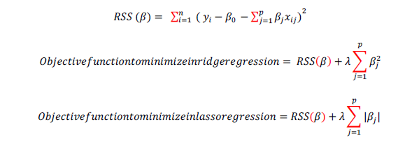
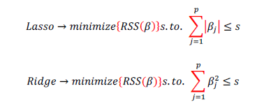
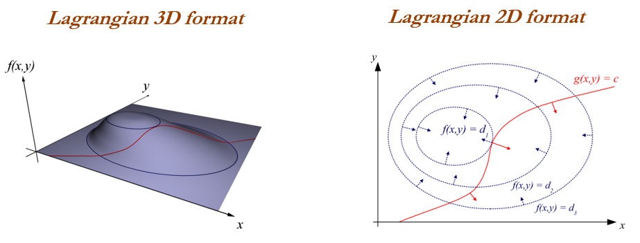
Before we go in deeper on ridge and lasso, it is worth to understand some concepts on Lagrangian multipliers. One can show the preceding objective function into the following format, where objective is just RSS subjected to cost constraint (s) of budget. For every value of λ, there is some s such that will provide the equivalent equations as shown as follows for overall objective function with penalty factor:

The following graph shows the two different Lagrangian format:

Ridge regression works well in situations where the least squares estimates have high variance. Ridge regression has computational advantages over best subset selection which required 2P models. In contrast for any fixed value of λ, ridge regression only fits a single model and model-fitting procedure can be performed very quickly.

One disadvantage of ridge regression is, it will include all the predictors and shrinks the weights according with its importance but it does not set the values exactly to zero in order to eliminate unnecessary predictors from models, this issue will be overcome in lasso regression. During the situation of number of predictors are significantly large, using ridge may provide good accuracy but it includes all the variables, which is not desired in compact representation of the model, this issue do not present in lasso as it will set the weights of unnecessary variables to zero.

Model generated from lasso are very much like subset selection, hence it is much easier to interpret than those produced by ridge regression.

Example of ridge regression machine learning model

Ridge regression is machine learning model, in which we do not perform any statistical diagnostics on the independent variables and just utilize the model to fit on test data and check the accuracy of fit. Here we have used scikit-learn package:

>>> from sklearn.linear_model import Ridge
>>> wine_quality = pd.read_csv(
>>> wine_quality.rename(columns=lambda x: x.replace(" ",
inplace=True)
>>> all_colnms = ['fixed_acidity', 'volatile_acidity',
'citric_acid', 'residual_sugar', 'chlorides',
Article_01.png
λ, ridge regression only fits a
idge exactly to zero in
egression. are significantly large,
idge variables, which is not
model, this issue do not present in lasso as it will
e regression machine learning model
learning model, in which we do not perform any statistical
the model to fit on test data and
have used scikit-learn package:
csv("winequality-red.csv",sep=';')
"_"),
in
ariables, asso odel
earning el
'free_sulfur_dioxide', 'total_sulfur_dioxide', 'density', 'pH',
'sulphates', 'alcohol']
>>> pdx = wine_quality[all_colnms]
>>> pdy = wine_quality["quality"]
>>> x_train,x_test,y_train,y_test =
train_test_split(pdx,pdy,train_size = 0.7,random_state=42)

Simple version of grid search from scratch has been described as follows, in which various values of alphas are tried to be tested in grid search to test the model fitness:

>>> alphas = [1e-4,1e-3,1e-2,0.1,0.5,1.0,5.0,10.0]

Initial values of R-squared are set to zero in order to keep track on its updated value and to print whenever new value is greater than exiting value:

>>> initrsq = 0
>>> print ("nRidge Regression: Best Parametersn")
>>> for alph in alphas:
... ridge_reg = Ridge(alpha=alph)
... ridge_reg.fit(x_train,y_train) 0
... tr_rsqrd = ridge_reg.score(x_train,y_train)
... ts_rsqrd = ridge_reg.score(x_test,y_test)

The following code always keep track on test R-squared value and prints if new value is greater than existing best value:

>>> if ts_rsqrd > initrsq:
... print ("Lambda: ",alph,"Train R-Squared
value:",round(tr_rsqrd,5),"Test R-squared
value:",round(ts_rsqrd,5))
... initrsq = ts_rsqrd

It is is shown in the following screenshot:

By looking into test R-squared (0.3513) value we can conclude that there is no significant relationship between independent and dependent variables.

Also, please note that, the test R-squared value generated from ridge regression is similar to value obtained from multiple linear regression (0.3519), but with the no stress on diagnostics of variables, and so on. Hence machine learning models are relatively compact and can be utilized for learning automatically without manual intervention to retrain the model, this is one of the biggest advantages of using ML models for deployment purposes.

The R code for ridge regression on wine quality data is shown as follows:

# Ridge regression
library(glmnet)
wine_quality = read.csv("winequality-red.csv",header=TRUE,sep =
";",check.names = FALSE)
names(wine_quality) <- gsub(" ", "_", names(wine_quality))
set.seed(123)
numrow = nrow(wine_quality)
trnind = sample(1:numrow,size = as.integer(0.7*numrow))
train_data = wine_quality[trnind,]; test_data = wine_quality[-
trnind,]
xvars =
c("fixed_acidity","volatile_acidity","citric_acid","residual_sugar
","chlorides","free_sulfur_dioxide",
"total_sulfur_dioxide","density","pH","sulphates","alcohol")
yvar = "quality"
x_train = as.matrix(train_data[,xvars]);y_train = as.double
(as.matrix (train_data[,yvar]))
x_test = as.matrix(test_data[,xvars])
print(paste("Ridge Regression"))
lambdas = c(1e-4,1e-3,1e-2,0.1,0.5,1.0,5.0,10.0)
initrsq = 0
for (lmbd in lambdas){
ridge_fit = glmnet(x_train,y_train,alpha = 0,lambda = lmbd)
pred_y = predict(ridge_fit,x_test)
R2 <- 1 - (sum((test_data[,yvar]-pred_y
)^2)/sum((test_data[,yvar]-mean(test_data[,yvar]))^2))
if (R2 > initrsq){
print(paste("Lambda:",lmbd,"Test Adjusted R-squared
:",round(R2,4)))
initrsq = R2
}
}

Example of lasso regression model

Lasso regression is close cousin of ridge regression, in which absolute values of coefficients are minimized rather than square of values. By doing so, we eliminate some insignificant variables, which are very much compacted representation similar to OLS methods.

Following implementation is almost similar to ridge regression apart from penalty application on mod/absolute value of coefficients:

>>> from sklearn.linear_model import Lasso
>>> alphas = [1e-4,1e-3,1e-2,0.1,0.5,1.0,5.0,10.0]
>>> initrsq = 0
>>> print ("nLasso Regression: Best Parametersn")
>>> for alph in alphas:
... lasso_reg = Lasso(alpha=alph)
... lasso_reg.fit(x_train,y_train)
... tr_rsqrd = lasso_reg.score(x_train,y_train)
... ts_rsqrd = lasso_reg.score(x_test,y_test)
... if ts_rsqrd > initrsq:
... print ("Lambda: ",alph,"Train R-Squared
value:",round(tr_rsqrd,5),"Test R-squared
value:",round(ts_rsqrd,5))
... initrsq = ts_rsqrd

It is shown in the following screenshot:

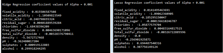
Lasso regression produces almost similar results as ridge, but if we check the test R-squared values bit carefully, lasso produces little less values. Reason behind the same could be due to its robustness of reducing coefficients to zero and eliminate them from analysis:

>>> ridge_reg = Ridge(alpha=0.001)
>>> ridge_reg.fit(x_train,y_train)
>>> print ("nRidge Regression coefficient values of Alpha =
0.001n")
>>> for i in range(11):
... print (all_colnms[i],": ",ridge_reg.coef_[i])
>>> lasso_reg = Lasso(alpha=0.001)
>>> lasso_reg.fit(x_train,y_train)
>>> print ("nLasso Regression coefficient values of Alpha =
0.001n")
>>> for i in range(11):
... print (all_colnms[i],": ",lasso_reg.coef_[i])

Following results shows the coefficient values of both the methods, coefficient of density has been set to o in lasso regression whereas density value is -5.5672 in ridge regression; also none of the coefficients in ridge regression are zero values:

R Code – Lasso Regression on Wine Quality Data

# Above Data processing steps are same as Ridge Regression, only
below section of the code do change
# Lasso Regression
print(paste("Lasso Regression"))
lambdas = c(1e-4,1e-3,1e-2,0.1,0.5,1.0,5.0,10.0)
initrsq = 0
for (lmbd in lambdas){
lasso_fit = glmnet(x_train,y_train,alpha = 1,lambda = lmbd)
pred_y = predict(lasso_fit,x_test)
R2 <- 1 - (sum((test_data[,yvar]-pred_y
)^2)/sum((test_data[,yvar]-mean(test_data[,yvar]))^2))
if (R2 > initrsq){
print(paste("Lambda:",lmbd,"Test Adjusted R-squared
:",round(R2,4)))
initrsq = R2
}
}

Regularization parameters in linear regression and ridge/lasso regression

Adjusted R-squared in linear regression always penalizes adding extra variables with less significance is one type of regularizing the data in linear regression, but it will adjust to unique fit of the model. Whereas in machine learning many parameters are adjusted to regularizing the overfitting problem, in the example of lasso/ridge regression penalty parameter (λ) to regularization, there are infinite values can be applied to regularize the model infinite ways:

In overall there are many similarities between statistical way and machine learning ways of predicting the pattern.

Summary

We have seen ridge regression and lasso regression with their examples and we have also seen its regularization parameters.

Resources for Article:

---

Further resources on this subject:

• Machine Learning Review [article]
• Getting Started with Python and Machine Learning [article]
• Machine learning in practice [article]

---