Clustering is one of the very important data mining and machine learning techniques. Clustering is a procedure for discovering groups of closely related elements in the dataset. Many a times we want to cluster the data into some categories, such as grouping similar users, modeling user behavior, identifying species of Irises, categorizing news items, classifying textual documents, and more. One of the most common clustering method is K-Means, which is a simple iterative method to partition the data into K - clusters.
Algorithm
Before we apply K-means to cluster data, it is required to express the data as vectors. In most of the cases, the data is given as a matrix of type [nSamples, nAttributes], which can be thought of as nSamples vectors each with a dimension of nAttributes.
There are certain cases where some work has to be done to render the data into linear algebraic language, such as:
A corpus of textual documents - We compute Term-frequency of a text document in the corpus as a vector of dimension=(vocabulary of the corpus) where the coefficient of each dimension is the frequency in the document of the word corresponding to the dimension.
There are other choices of creating vectors from text documents, such as TFIDF vectors, binary vectors and more.
If I'm trying to cluster by Twitter friends, I can represent each friend as a vector:
number of followers, number of friends, number of tweets, count of favorite tweets
After we have vectors representing data points, we will cluster these data vectors into K clusters using the following algorithm.
Initialize the procedure by randomly selecting K vectors as cluster centroids.
For each vector compute its Euclidean distance with each of the centroids and assign the vector to its closest centroid.
When all of the objects have been assigned, recalculate the centroids as the mean (average) of all members of the cluster.
Repeat the previous two steps until convergence – when the clusters no longer change.
You can also choose other distance measures such as: Cosine similarity, Pearson correlation, Manhatten distance, and so on.
Example
We'll do cluster analysis of the wine dataset. This data contains 13 chemical measurements on 178 Italian wine samples. The data is taken from the UCI Machine Learning Repository. I'll use R to do this analysis, but it can very easily be done in other programing languages such as Python.
We'll use the R package rattle, which is GUI for data mining in R. We use rattle only to access data from the UCI Machine Learning Repository.
The first column contains the types of the wine. We will use K-Means as a learning model to predict the types:
# remove te first column
input <- scale(wine[-1])
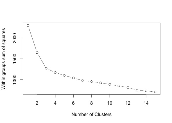
A drawback of K-means clustering is that we have to pre-decide on the number of clusters. First, we'll define a function to compute the optimal number of clusters by looking at the clusters sum of squares for a different number of clusters.
wssplot <- function(data, nc=15, seed=1234){
wss <- (nrow(data)-1)*sum(apply(data,2,var))
for (i in 2:nc){
set.seed(seed)
wss[i] <- sum(kmeans(data, centers=i)$withinss)}
plot(1:nc, wss, type="b", xlab="Number of Clusters",
ylab="Within groups sum of squares")}
Now we'll compute the optimal number of clusters using the wss function we defined above:
pdf("Number of Clusters.pdf")
wssplot(input)
dev.off()
The plot shows within groups the sums of squares vs. the number of clusters extracted. The sharp decreases from 1 to 3 clusters (with a little decrease after) suggesting a 3-cluster solution. This shows that the optimal number of clusters is 3.
Now we will cluster the data into 3 clusters using the kmeans() function in R.
set.seed(1234)
# Clusters
fit <- kmeans(input, 3, nstart=25)
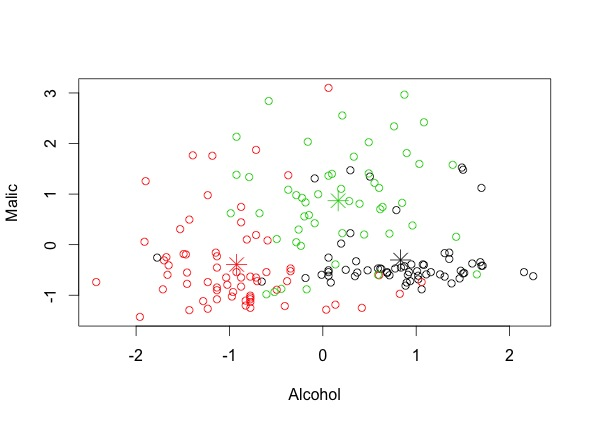
Let's plot the clusters:
Unlock access to the largest independent learning library in Tech for FREE!
Get unlimited access to 7500+ expert-authored eBooks and video courses covering every tech area you can think of.
# Size of the Clusters
size <- fit$size
size
>>> [1] 62 65 51
Thus we have three clusters of wines of size 62, 65 and 51.
The means of the columns (chemicals) for each of the cluster can be computed using the aggregate function.
# Means of the columns for the Clusters
mean_coulmns <- aggregate(input, by=list(fit$cluster), FUN=mean)
mean_columns
Let's now measure how good this clustering is. We can use K-Means as a predictive model to assign new data points to one of the 3 clusters. First, we should check how well this assignment is for the training set.
A metric for this evaluation is called Cross Tabulation. This is a table comparing the type assigned by clustering and original values.
# Measuring How Good is the Clustering
# Cross Tabulation : A table comparing type assigned by clustering and original values
cross <- table(wine$Type, fit$cluster)
cross
>>>
1 2 3
1 59 0 0
2 3 65 3
3 0 0 48
This shows that the clustering gives a pretty good prediction.
Want more Machine Learning tutorials and content? Visit our dedicated Machine Learning page here.
About the Author
Janu Verma is a Quantitative Researcher at the Buckler Lab, Cornell University, where he works on problems in bioinformatics and genomics. His background is in mathematics and machine learning and he leverages tools from these areas to answer questions in biology.

 United States
 Great Britain
 India
India
 Germany
 France
 Canada
 Russia
 Spain
Spain
 Brazil
 Australia
 Singapore
 Canary Islands
 Hungary
 Ukraine
 Luxembourg
 Estonia
 Lithuania
 South Korea
 Turkey
 Switzerland
 Colombia
 Taiwan
 Chile
Chile
 Norway
 Ecuador
 Indonesia
 New Zealand
 Cyprus
 Denmark
 Finland
 Poland
 Malta
Malta
 Czechia
 Austria
 Sweden
 Italy
Italy
 Egypt
Egypt
 Belgium
 Portugal
 Slovenia
 Ireland
 Romania
 Greece
 Argentina
 Netherlands
 Bulgaria
 Latvia
 South Africa
 Malaysia
 Japan
Japan
 Slovakia
 Philippines
 Mexico
 Thailand