Introduction to Clustering and Unsupervised Learning
Read more
Introduction to Clustering and Unsupervised Learning
Packt
960 min read
2016-02-23 00:00:00
0 Likes
0 Comments
The act of clustering, or spotting patterns in data, is not much different from spotting patterns in groups of people. In this article, you will learn:
The ways clustering tasks differ from the classification tasks
How clustering defines a group, and how such groups are identified by k-means, a classic and easy-to-understand clustering algorithm
The steps needed to apply clustering to a real-world task of identifying marketing segments among teenage social media users
Before jumping into action, we'll begin by taking an in-depth look at exactly what clustering entails.
(For more resources related to this topic, see here.)
Understanding clustering
Clustering is an unsupervised machine learning task that automatically divides the data into clusters, or groups of similar items. It does this without having been told how the groups should look ahead of time. As we may not even know what we're looking for, clustering is used for knowledge discovery rather than prediction. It provides an insight into the natural groupings found within data.
Without advance knowledge of what comprises a cluster, how can a computer possibly know where one group ends and another begins? The answer is simple. Clustering is guided by the principle that items inside a cluster should be very similar to each other, but very different from those outside. The definition of similarity might vary across applications, but the basic idea is always the same—group the data so that the related elements are placed together.
The resulting clusters can then be used for action. For instance, you might find clustering methods employed in the following applications:
Segmenting customers into groups with similar demographics or buying patterns for targeted marketing campaigns
Detecting anomalous behavior, such as unauthorized network intrusions, by identifying patterns of use falling outside the known clusters
Simplifying extremely large datasets by grouping features with similar values into a smaller number of homogeneous categories
Overall, clustering is useful whenever diverse and varied data can be exemplified by a much smaller number of groups. It results in meaningful and actionable data structures that reduce complexity and provide insight into patterns of relationships.
Clustering as a machine learning task
Clustering is somewhat different from the classification, numeric prediction, and pattern detection tasks we examined so far. In each of these cases, the result is a model that relates features to an outcome or features to other features; conceptually, the model describes the existing patterns within data. In contrast, clustering creates new data. Unlabeled examples are given a cluster label that has been inferred entirely from the relationships within the data. For this reason, you will, sometimes, see the clustering task referred to as unsupervised classification because, in a sense, it classifies unlabeled examples.
The catch is that the class labels obtained from an unsupervised classifier are without intrinsic meaning. Clustering will tell you which groups of examples are closely related—for instance, it might return the groups A, B, and C—but it's up to you to apply an actionable and meaningful label. To see how this impacts the clustering task, let's consider a hypothetical example.
Suppose you were organizing a conference on the topic of data science. To facilitate professional networking and collaboration, you planned to seat people in groups according to one of three research specialties: computer and/or database science, math and statistics, and machine learning. Unfortunately, after sending out the conference invitations, you realize that you had forgotten to include a survey asking which discipline the attendee would prefer to be seated with.
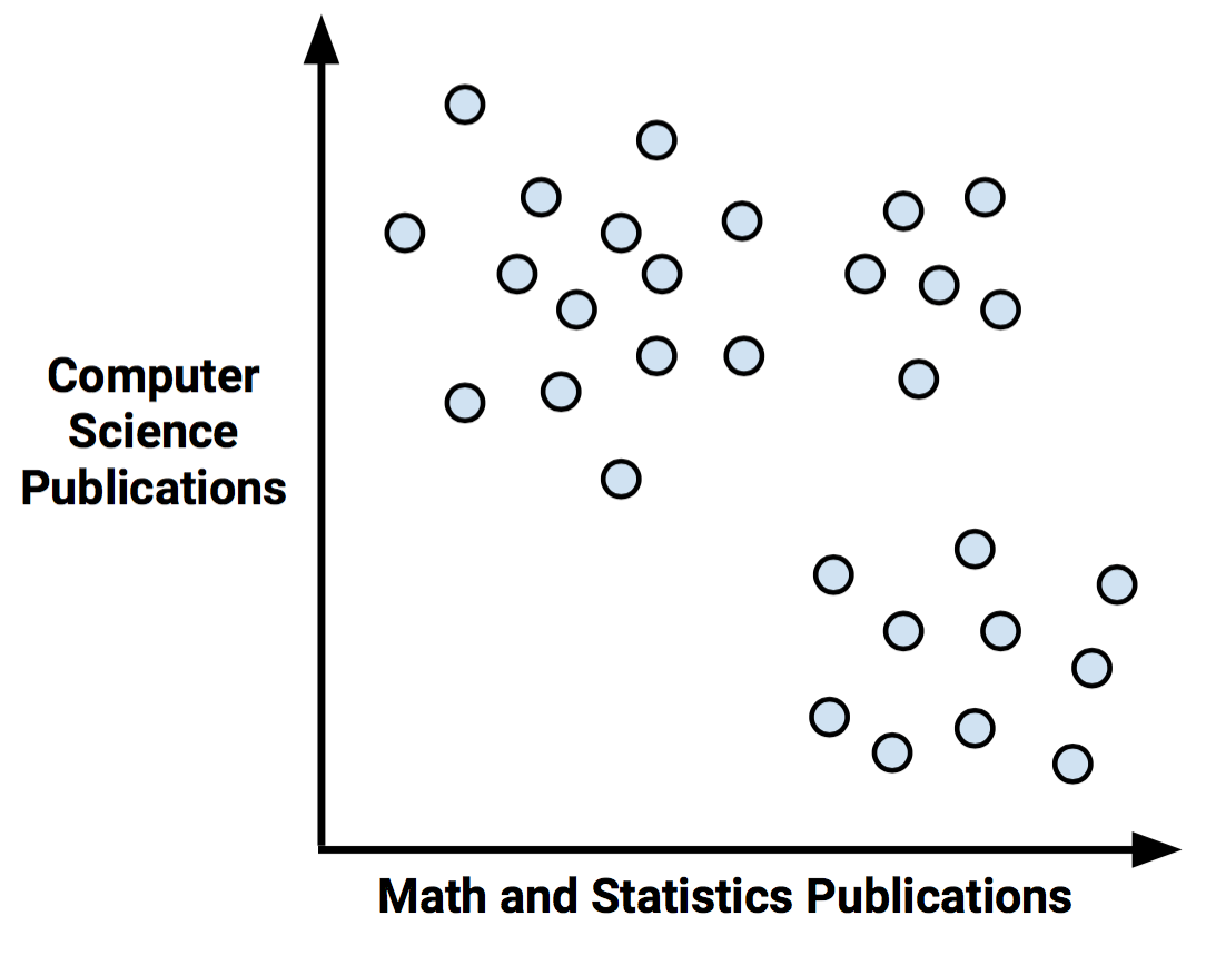
In a stroke of brilliance, you realize that you might be able to infer each scholar's research specialty by examining his or her publication history. To this end, you begin collecting data on the number of articles each attendee published in computer science-related journals and the number of articles published in math or statistics-related journals. Using the data collected for several scholars, you create a scatterplot:
As expected, there seems to be a pattern. We might guess that the upper-left corner, which represents people with many computer science publications but few articles on math, could be a cluster of computer scientists. Following this logic, the lower-right corner might be a group of mathematicians. Similarly, the upper-right corner, those with both math and computer science experience, may be machine learning experts.
Our groupings were formed visually; we simply identified clusters as closely grouped data points. Yet in spite of the seemingly obvious groupings, we unfortunately have no way to know whether they are truly homogeneous without personally asking each scholar about his/her academic specialty. The labels we applied required us to make qualitative, presumptive judgments about the types of people that would fall into the group. For this reason, you might imagine the cluster labels in uncertain terms, as follows:
Rather than defining the group boundaries subjectively, it would be nice to use machine learning to define them objectively. This might provide us with a rule in the form if a scholar has few math publications, then he/she is a computer science expert. Unfortunately, there's a problem with this plan. As we do not have data on the true class value for each point, a supervised learning algorithm would have no ability to learn such a pattern, as it would have no way of knowing what splits would result in homogenous groups.
On the other hand, clustering algorithms use a process very similar to what we did by visually inspecting the scatterplot. Using a measure of how closely the examples are related, homogeneous groups can be identified. In the next section, we'll start looking at how clustering algorithms are implemented.
This example highlights an interesting application of clustering. If you begin with unlabeled data, you can use clustering to create class labels. From there, you could apply a supervised learner such as decision trees to find the most important predictors of these classes. This is called semi-supervised learning.
The k-means clustering algorithm
The k-means algorithm is perhaps the most commonly used clustering method. Having been studied for several decades, it serves as the foundation for many more sophisticated clustering techniques. If you understand the simple principles it uses, you will have the knowledge needed to understand nearly any clustering algorithm in use today. Many such methods are listed on the following site, the CRAN Task View for clustering at http://cran.r-project.org/web/views/Cluster.html.
As k-means has evolved over time, there are many implementations of the algorithm. One popular approach is described in : Hartigan JA, Wong MA. A k-means clustering algorithm. Applied Statistics. 1979; 28:100-108.
Even though clustering methods have advanced since the inception of k-means, this is not to imply that k-means is obsolete. In fact, the method may be more popular now than ever. The following table lists some reasons why k-means is still used widely:
Strengths
Weaknesses
Uses simple principles that can be explained in non-statistical terms
Highly flexible, and can be adapted with simple adjustments to address nearly all of its shortcomings
Performs well enough under many real-world use cases
Not as sophisticated as more modern clustering algorithms
Because it uses an element of random chance, it is not guaranteed to find the optimal set of clusters
Requires a reasonable guess as to how many clusters naturally exist in the data
Not ideal for non-spherical clusters or clusters of widely varying density
The k-means algorithm assigns each of the n examples to one of the k clusters, where k is a number that has been determined ahead of time. The goal is to minimize the differences within each cluster and maximize the differences between the clusters.
Unless k and n are extremely small, it is not feasible to compute the optimal clusters across all the possible combinations of examples. Instead, the algorithm uses a heuristic process that finds locally optimal solutions. Put simply, this means that it starts with an initial guess for the cluster assignments, and then modifies the assignments slightly to see whether the changes improve the homogeneity within the clusters.
We will cover the process in depth shortly, but the algorithm essentially involves two phases. First, it assigns examples to an initial set of k clusters. Then, it updates the assignments by adjusting the cluster boundaries according to the examples that currently fall into the cluster. The process of updating and assigning occurs several times until changes no longer improve the cluster fit. At this point, the process stops and the clusters are finalized.
Due to the heuristic nature of k-means, you may end up with somewhat different final results by making only slight changes to the starting conditions. If the results vary dramatically, this could indicate a problem. For instance, the data may not have natural groupings or the value of k has been poorly chosen. With this in mind, it's a good idea to try a cluster analysis more than once to test the robustness of your findings.
To see how the process of assigning and updating works in practice, let's revisit the case of the hypothetical data science conference. Though this is a simple example, it will illustrate the basics of how k-means operates under the hood.
Using distance to assign and update clusters
As with k-NN, k-means treats feature values as coordinates in a multidimensional feature space. For the conference data, there are only two features, so we can represent the feature space as a two-dimensional scatterplot as depicted previously.
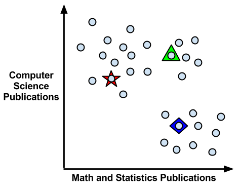
The k-means algorithm begins by choosing k points in the feature space to serve as the cluster centers. These centers are the catalyst that spurs the remaining examples to fall into place. Often, the points are chosen by selecting k random examples from the training dataset. As we hope to identify three clusters, according to this method, k = 3 points will be selected at random. These points are indicated by the star, triangle, and diamond in the following diagram:
It's worth noting that although the three cluster centers in the preceding diagram happen to be widely spaced apart, this is not always necessarily the case. Since they are selected at random, the three centers could have just as easily been three adjacent points. As the k-means algorithm is highly sensitive to the starting position of the cluster centers, this means that random chance may have a substantial impact on the final set of clusters.
To address this problem, k-means can be modified to use different methods for choosing the initial centers. For example, one variant chooses random values occurring anywhere in the feature space (rather than only selecting among the values observed in the data). Another option is to skip this step altogether; by randomly assigning each example to a cluster, the algorithm can jump ahead immediately to the update phase. Each of these approaches adds a particular bias to the final set of clusters, which you may be able to use to improve your results.
Unlock access to the largest independent learning library in Tech for FREE!
Get unlimited access to 7500+ expert-authored eBooks and video courses covering every tech area you can think of.
Renews at $19.99/month. Cancel anytime
In 2007, an algorithm called k-means++ was introduced, which proposes an alternative method for selecting the initial cluster centers. It purports to be an efficient way to get much closer to the optimal clustering solution while reducing the impact of random chance. For more information, refer to Arthur D, Vassilvitskii S. k-means++: The advantages of careful seeding. Proceedings of the eighteenth annual ACM-SIAM symposium on discrete algorithms. 2007:1027–1035.
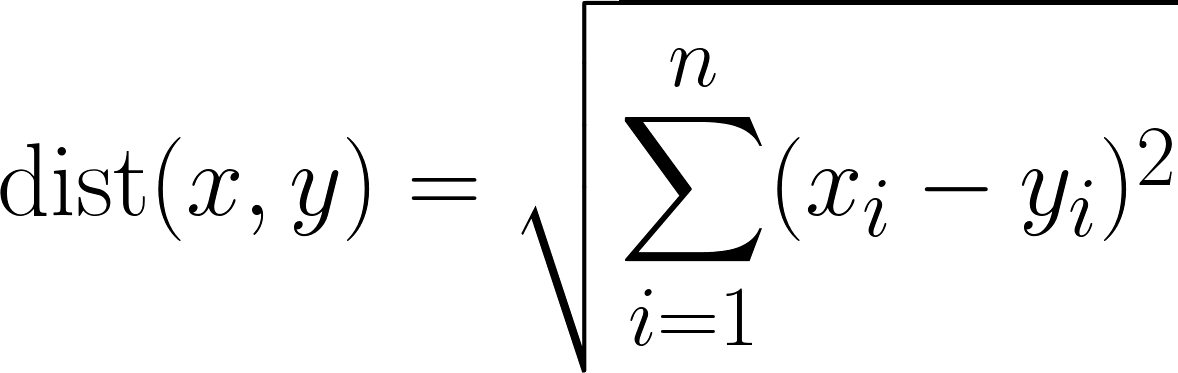
After choosing the initial cluster centers, the other examples are assigned to the cluster center that is nearest according to the distance function. You will remember that we studied distance functions while learning about k-Nearest Neighbors. Traditionally, k-means uses Euclidean distance, but Manhattan distance or Minkowski distance are also sometimes used.
Recall that if n indicates the number of features, the formula for Euclidean distance between example x and example y is:
For instance, if we are comparing a guest with five computer science publications and one math publication to a guest with zero computer science papers and two math papers, we could compute this in R as follows:
> sqrt((5 - 0)^2 + (1 - 2)^2)
[1] 5.09902
Using this distance function, we find the distance between each example and each cluster center. The example is then assigned to the nearest cluster center.
Keep in mind that as we are using distance calculations, all the features need to be numeric, and the values should be normalized to a standard range ahead of time.
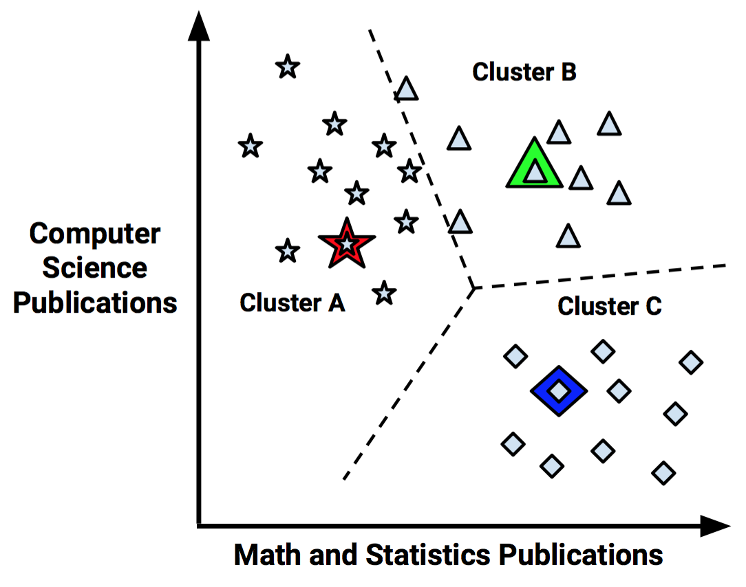
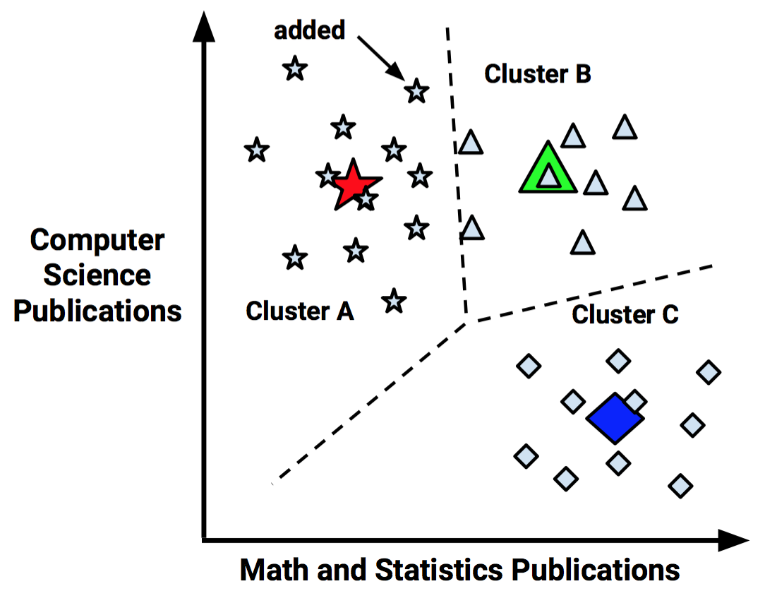
As shown in the following diagram, the three cluster centers partition the examples into three segments labeled Cluster A, Cluster B, and Cluster C. The dashed lines indicate the boundaries for the Voronoi diagram created by the cluster centers. The Voronoi diagram indicates the areas that are closer to one cluster center than any other; the vertex where all the three boundaries meet is the maximal distance from all three cluster centers. Using these boundaries, we can easily see the regions claimed by each of the initial k-means seeds:
Now that the initial assignment phase has been completed, the k-means algorithm proceeds to the update phase. The first step of updating the clusters involves shifting the initial centers to a new location, known as the centroid, which is calculated as the average position of the points currently assigned to that cluster. The following diagram illustrates how as the cluster centers shift to the new centroids, the boundaries in the Voronoi diagram also shift and a point that was once in Cluster B (indicated by an arrow) is added to Cluster A:
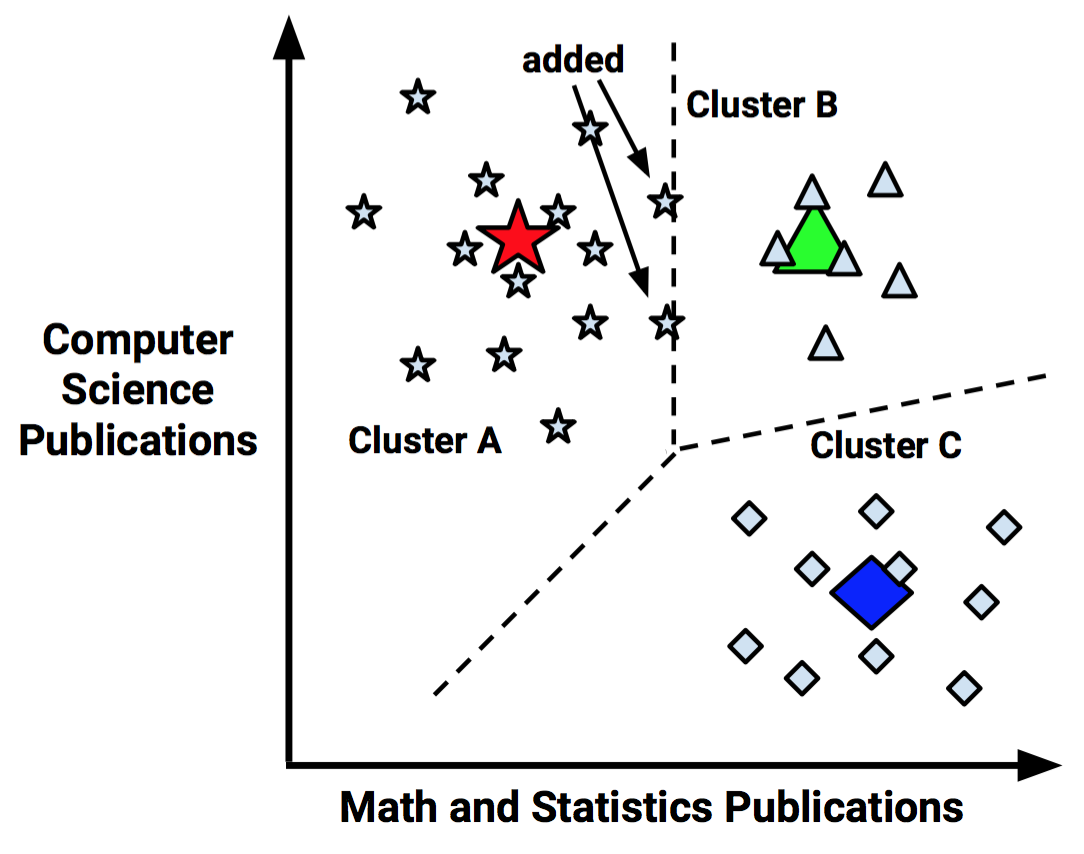
As a result of this reassignment, the k-means algorithm will continue through another update phase. After shifting the cluster centroids, updating the cluster boundaries, and reassigning points into new clusters (as indicated by arrows), the figure looks like this:
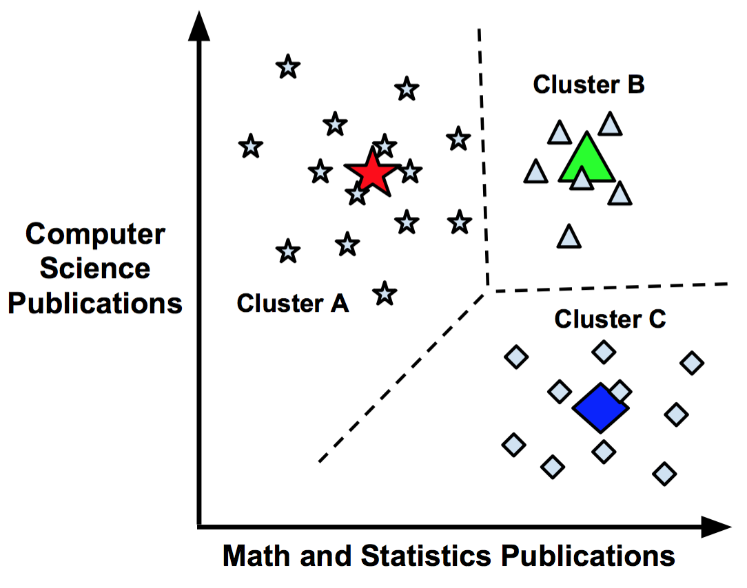
Because two more points were reassigned, another update must occur, which moves the centroids and updates the cluster boundaries. However, because these changes result in no reassignments, the k-means algorithm stops. The cluster assignments are now final:
The final clusters can be reported in one of the two ways. First, you might simply report the cluster assignments such as A, B, or C for each example. Alternatively, you could report the coordinates of the cluster centroids after the final update. Given either reporting method, you are able to define the cluster boundaries by calculating the centroids or assigning each example to its nearest cluster.
Choosing the appropriate number of clusters
In the introduction to k-means, we learned that the algorithm is sensitive to the randomly-chosen cluster centers. Indeed, if we had selected a different combination of three starting points in the previous example, we may have found clusters that split the data differently from what we had expected. Similarly, k-means is sensitive to the number of clusters; the choice requires a delicate balance. Setting k to be very large will improve the homogeneity of the clusters, and at the same time, it risks overfitting the data.
Ideally, you will have a priori knowledge (a prior belief) about the true groupings and you can apply this information to choosing the number of clusters. For instance, if you were clustering movies, you might begin by setting k equal to the number of genres considered for the Academy Awards. In the data science conference seating problem that we worked through previously, k might reflect the number of academic fields of study that were invited.
Sometimes the number of clusters is dictated by business requirements or the motivation for the analysis. For example, the number of tables in the meeting hall could dictate how many groups of people should be created from the data science attendee list. Extending this idea to another business case, if the marketing department only has resources to create three distinct advertising campaigns, it might make sense to set k = 3 to assign all the potential customers to one of the three appeals.
Without any prior knowledge, one rule of thumb suggests setting k equal to the square root of (n / 2), where n is the number of examples in the dataset. However, this rule of thumb is likely to result in an unwieldy number of clusters for large datasets. Luckily, there are other statistical methods that can assist in finding a suitable k-means cluster set.
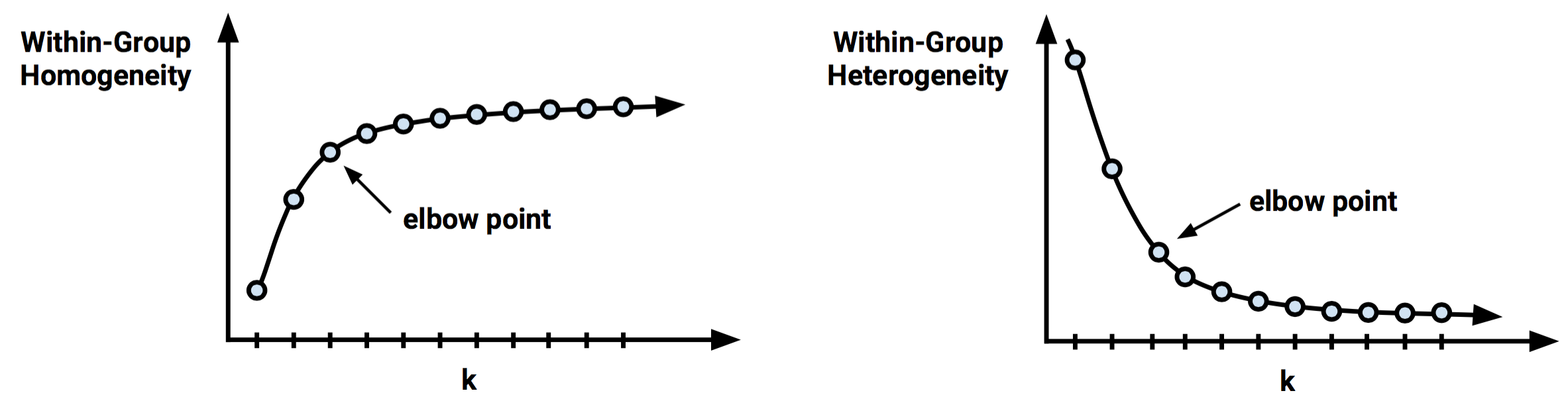
A technique known as the elbow method attempts to gauge how the homogeneity or heterogeneity within the clusters changes for various values of k. As illustrated in the following diagrams, the homogeneity within clusters is expected to increase as additional clusters are added; similarly, heterogeneity will also continue to decrease with more clusters. As you could continue to see improvements until each example is in its own cluster, the goal is not to maximize homogeneity or minimize heterogeneity, but rather to find k so that there are diminishing returns beyond that point. This value of k is known as the elbow point because it looks like an elbow.
There are numerous statistics to measure homogeneity and heterogeneity within the clusters that can be used with the elbow method (the following information box provides a citation for more detail). Still, in practice, it is not always feasible to iteratively test a large number of k values. This is in part because clustering large datasets can be fairly time consuming; clustering the data repeatedly is even worse. Regardless, applications requiring the exact optimal set of clusters are fairly rare. In most clustering applications, it suffices to choose a k value based on convenience rather than strict performance requirements.
For a very thorough review of the vast assortment of cluster performance measures, refer to: Halkidi M, Batistakis Y, Vazirgiannis M. On clustering validation techniques. Journal of Intelligent Information Systems. 2001; 17:107-145.
The process of setting k itself can sometimes lead to interesting insights. By observing how the characteristics of the clusters change as k is varied, one might infer where the data have naturally defined boundaries. Groups that are more tightly clustered will change a little, while less homogeneous groups will form and disband over time.
In general, it may be wise to spend little time worrying about getting k exactly right. The next example will demonstrate how even a tiny bit of subject-matter knowledge borrowed from a Hollywood film can be used to set k such that actionable and interesting clusters are found. As clustering is unsupervised, the task is really about what you make of it; the value is in the insights you take away from the algorithm's findings.
Summary
This article covered only the fundamentals of clustering. As a very mature machine learning method, there are many variants of the k-means algorithm as well as many other clustering algorithms that bring unique biases and heuristics to the task. Based on the foundation in this article, you will be able to understand and apply other clustering methods to new problems.
To learn more about different machine learning techniques, the following books published by Packt Publishing (https://www.packtpub.com/) are recommended:
Learning Data Mining with R (https://www.packtpub.com/big-data-and-business-intelligence/learning-data-mining-r)
Mastering Scientific Computing with R (https://www.packtpub.com/application-development/mastering-scientific-computing-r)
R for Data Science (https://www.packtpub.com/big-data-and-business-intelligence/r-data-science)

 United States
 Great Britain
 India
India
 Germany
 France
 Canada
 Russia
 Spain
Spain
 Brazil
 Australia
 Singapore
 Canary Islands
 Hungary
 Ukraine
 Luxembourg
 Estonia
 Lithuania
 South Korea
 Turkey
 Switzerland
 Colombia
 Taiwan
 Chile
Chile
 Norway
 Ecuador
 Indonesia
 New Zealand
 Cyprus
 Denmark
 Finland
 Poland
 Malta
Malta
 Czechia
 Austria
 Sweden
 Italy
Italy
 Egypt
Egypt
 Belgium
 Portugal
 Slovenia
 Ireland
 Romania
 Greece
 Argentina
 Netherlands
 Bulgaria
 Latvia
 South Africa
 Malaysia
 Japan
Japan
 Slovakia
 Philippines
 Mexico
 Thailand