Implementing 3 Naive Bayes classifiers in scikit-learn

Scikit-learn provide three naive Bayes implementations: Bernoulli, multinomial and Gaussian. The only difference is about the probability distribution adopted. The first one is a binary algorithm particularly useful when a feature can be present or not. Multinomial naive Bayes assumes to have feature vector where each element represents the number of times it appears (or, very often, its frequency). This technique is very efficient in natural language processing or whenever the samples are composed starting from a common dictionary. The Gaussian Naive Bayes, instead, is based on a continuous distribution and it’s suitable for more generic classification tasks.

Ok, now that we have established naive Bayes variants are a handy set of algorithms to have in our machine learning arsenal and that Scikit-learn is a good tool to implement them, let’s rewind a bit.

What is Naive Bayes?

Naive Bayes are a family of powerful and easy-to-train classifiers, which determine the probability of an outcome, given a set of conditions using the Bayes’ theorem. In other words, the conditional probabilities are inverted so that the query can be expressed as a function of measurable quantities. The approach is simple and the adjective naive has been attributed not because these algorithms are limited or less efficient, but because of a fundamental assumption about the causal factors that we will discuss.

Naive Bayes are multi-purpose classifiers and it’s easy to find their application in many different contexts. However, the performance is particularly good in all those situations when the probability of a class is determined by the probabilities of some causal factors. A good example is given by natural language processing, where a text can be considered as a particular instance of a dictionary and the relative frequencies of all terms provide enough information to infer a belonging class. Our examples may be generic, so to let you understand the application of naive Bayes in various context.

The Bayes’ theorem

Let’s consider two probabilistic events A and B. We can correlate the marginal probabilities P(A) and P(B) with the conditional probabilities P(A|B) and P(B|A) using the product rule:

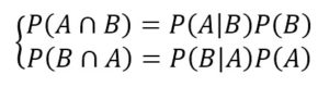
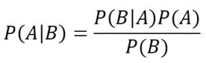
Considering that the intersection is commutative, the first members are equal, so we can derive the Bayes’ theorem:

This formula has very deep philosophical implications and it’s a fundamental element of statistical learning. First of all, let’s consider the marginal probability P(A): this is normally a value that determines how probable a target event is, like P(Spam) or P(Rain). As there are no other elements, this kind of probability is called Apriori, because it’s often determined by mathematical considerations or simply by a frequency count. For example, imagine we want to implement a very simple spam filter and we’ve collected 100 emails. We know that 30 are spam and 70 are regular. So we can say that P(Spam) = 0.3.

However, we’d like to evaluate using some criteria (for simplicity, let’s consider a single one), for example, e-mail text is shorter than 50 characters. Therefore, our query becomes:

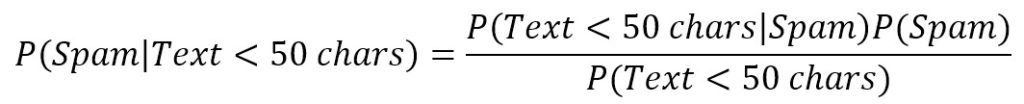
The first term is similar to P(Spam) because it’s the probability of spam given a certain condition. For this reason, it’s called a posteriori (in other words, it’s a probability that can estimate after knowing some additional elements). On the right side, we need to calculate the missing values, but it’s simple. Let’s suppose that 35 emails have a text shorter than 50 characters, P(Text < 50 chars) = 0.35 and, looking only into our spam folder, we discover that only 25 spam emails have a short text, so that P(Text < 50 chars|Spam) = 25/30 = 0.83. The result is:

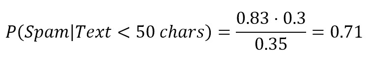
So, after receiving a very short email, there is 71% probability that it’s a spam. Now we can understand the role of P(Text < 50 chars|Spam): as we have actual data, we can measure how probable is our hypothesis given the query, in other words, we have defined a likelihood (compare this with logistic regression) which is a weight between the Apriori probability and the a posteriori one (the term on the denominator is less important because it works as normalizing factor):

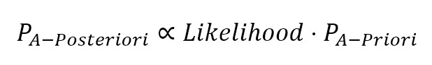
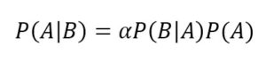
The normalization factor is often represented by the Greek letter alpha, so the formula becomes:

The last step is considering the case when there are more concurrent conditions (that is more realistic in real-life problems):

A common assumption is called conditional independence (in other words, the effects produced by every cause are independent among each other) and allows us to write a simplified expression:

Naive Bayes classifiers

A naive Bayes classifier is called in this way because it’s based on a naive condition, which implies the conditional independence of causes. This can seem very difficult to accept in many contexts where the probability of a particular feature is strictly correlated to another one. For example, in spam filtering, a text shorter than 50 characters can increase the probability of the presence of an image, or if the domain has been already blacklisted for sending the same spam emails to million users, it’s likely to find particular keywords. In other words, the presence of a cause isn’t normally independent from the presence of other ones. However, in Zhang H., The Optimality of Naive Bayes, AAAI 1, no. 2 (2004): 3, the author showed that under particular conditions (not so rare to happen), different dependencies clears one another, and a naive Bayes classifier succeeds in achieving very high performances even if its naiveness is violated.

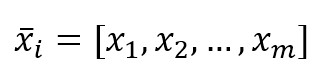
Let’s consider a dataset:

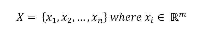
Every feature vector, for simplicity, will be represented as:

We need also a target dataset:

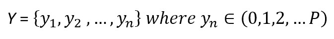
where each y can belong to one of P different classes. Considering the Bayes’ theorem under conditional independence, we can write:

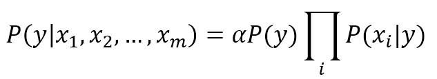
The values of the marginal Apriori probability P(y) and of the conditional probabilities P(xi|y) is obtained through a frequency count, therefore, given an input vector x, the predicted class is the one which a posteriori probability is maximum.

Naive Bayes in scikit-learn

scikit-learn implements three naive Bayes variants based on the same number of different probabilistic distributions: Bernoulli, multinomial, and Gaussian. The first one is a binary distribution useful when a feature can be present or absent. The second one is a discrete distribution used whenever a feature must be represented by a whole number (for example, in natural language processing, it can be the frequency of a term), while the latter is a continuous distribution characterized by its mean and variance.

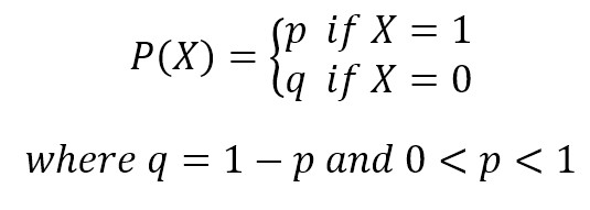
Bernoulli naive Bayes

If X is random variable Bernoulli-distributed, it can assume only two values (for simplicity, let’s call them 0 and 1) and their probability is:

To try this algorithm with scikit-learn, we’re going to generate a dummy dataset. Bernoulli naive Bayes expects binary feature vectors, however, the class BernoulliNB has a binarize parameter which allows specifying a threshold that will be used internally to transform the features:

from sklearn.datasets import make_classification

>>> nb_samples = 300
>>> X, Y = make_classification(n_samples=nb_samples, n_features=2, n_informative=2, n_redundant=0)

We have a generated the bidimensional dataset shown in the following figure:

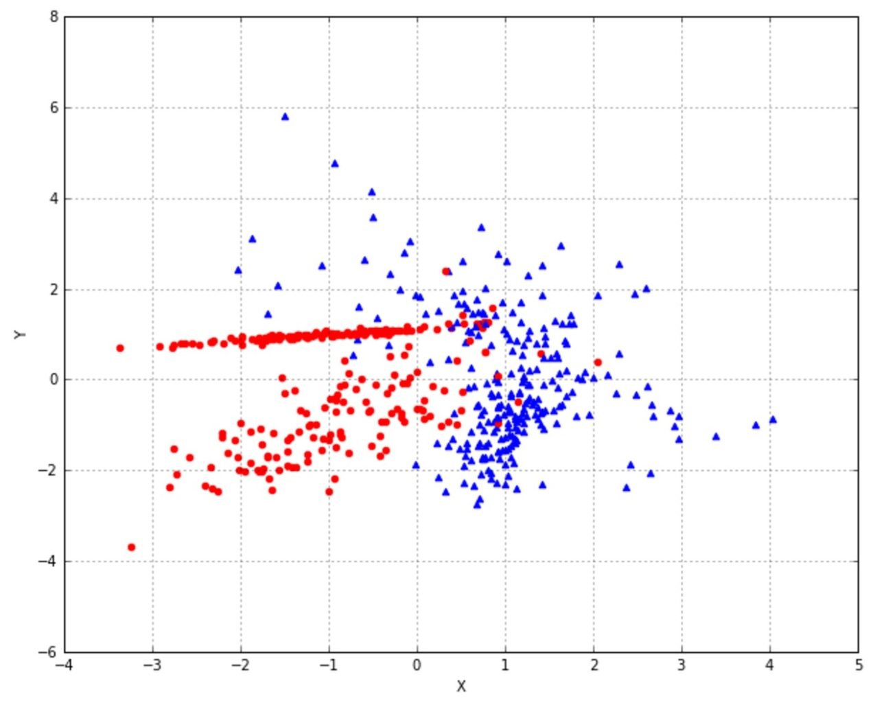
We have decided to use 0.0 as a binary threshold, so each point can be characterized by the quadrant where it’s located. Of course, this is a rational choice for our dataset, but Bernoulli naive Bayes is thought for binary feature vectors or continuous values which can be precisely split with a predefined threshold.

from sklearn.naive_bayes import BernoulliNB
from sklearn.model_selection import train_test_split

>>> X_train, X_test, Y_train, Y_test = train_test_split(X, Y, test_size=0.25)

>>> bnb = BernoulliNB(binarize=0.0)
>>> bnb.fit(X_train, Y_train)
>>> bnb.score(X_test, Y_test)
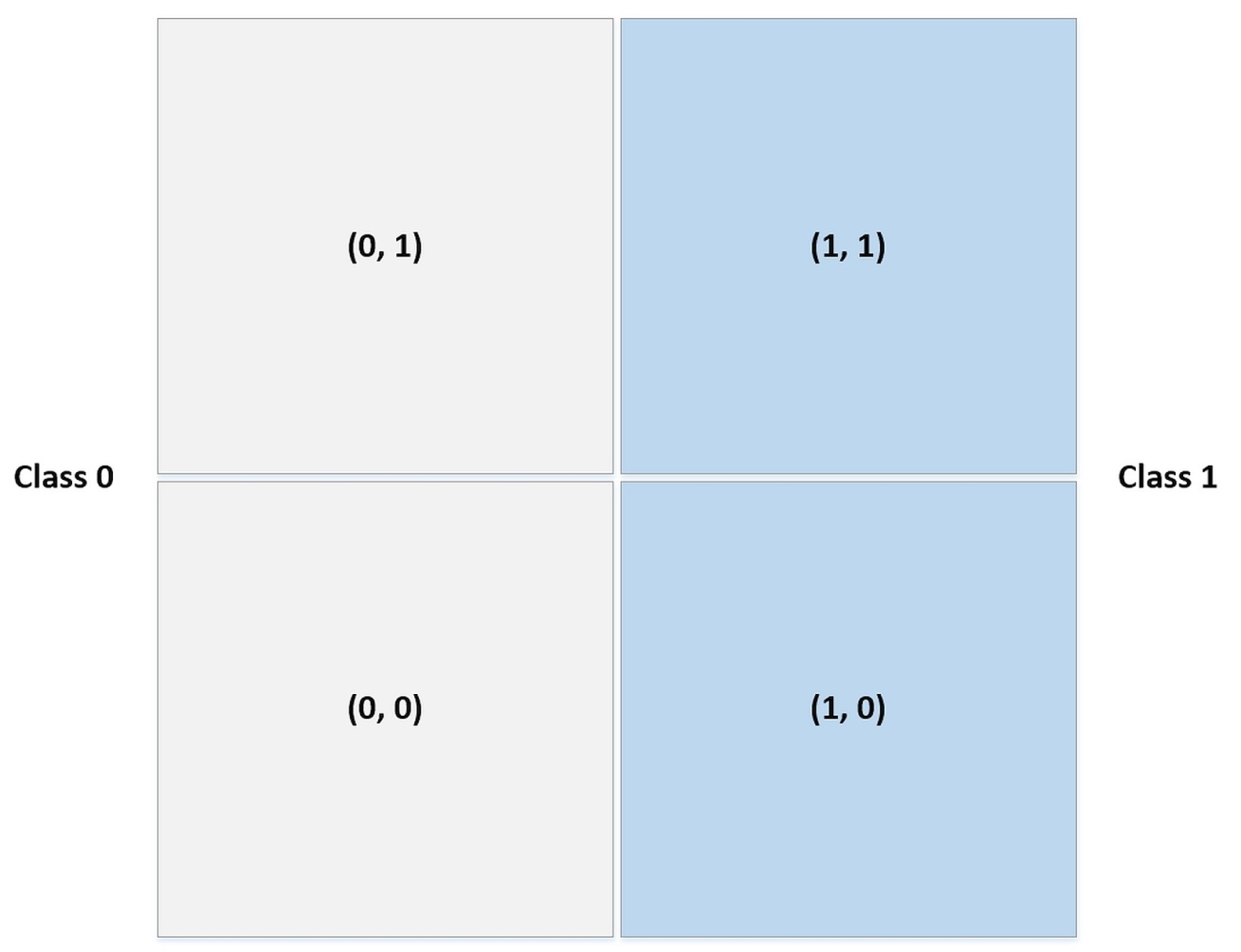
0.85333333333333339

The score in rather good, but if we want to understand how the binary classifier worked, it’s useful to see how the data have been internally binarized:

Now, checking the naive Bayes predictions we obtain:

>>> data = np.array([[0, 0], [0, 1], [1, 0], [1, 1]])
>>> bnb.predict(data)
array([0, 0, 1, 1])

Which is exactly what we expected.

Multinomial naive Bayes

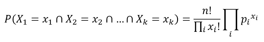
A multinomial distribution is useful to model feature vectors where each value represents, for example, the number of occurrences of a term or its relative frequency. If the feature vectors have n elements and each of them can assume k different values with probability pk, then:

The conditional probabilities P(xi|y) are computed with a frequency count (which corresponds to applying a maximum likelihood approach), but in this case, it’s important to consider the alpha parameter (called Laplace smoothing factor) which default value is 1.0 and prevents the model from setting null probabilities when the frequency is zero. It’s possible to assign all non-negative values, however, larger values will assign higher probabilities to the missing features and this choice could alter the stability of the model. In our example, we’re going to consider the default value of 1.0.

For our purposes, we’re going to use the DictVectorizer. There are automatic instruments to compute the frequencies of terms, but we’re going to discuss them later. Let’s consider only two records: the first one representing a city, while the second one countryside. Our dictionary contains hypothetical frequencies, like if the terms were extracted from a text description:

from sklearn.feature_extraction import DictVectorizer

>>> data = [
{'house': 100, 'street': 50, 'shop': 25, 'car': 100, 'tree': 20},

{'house': 5, 'street': 5, 'shop': 0, 'car': 10, 'tree': 500, 'river': 1}
] 

>>> dv = DictVectorizer(sparse=False)
>>> X = dv.fit_transform(data)
>>> Y = np.array([1, 0])

>>> X
array([[ 100.,  100.,    0.,   25.,   50.,   20.],
[  10.,    5.,    1.,    0.,    5.,  500.]])

Note that the term ‘river’ is missing from the first set, so it’s useful to keep alpha equal to 1.0 to give it a small probability. The output classes are 1 for city and 0 for the countryside. Now we can train a MultinomialNB instance:

from sklearn.naive_bayes import MultinomialNB

>>> mnb = MultinomialNB()
>>> mnb.fit(X, Y)
MultinomialNB(alpha=1.0, class_prior=None, fit_prior=True)

To test the model, we create a dummy city with a river and a dummy country place without any river.

>>> test_data = data = [
{'house': 80, 'street': 20, 'shop': 15, 'car': 70, 'tree': 10, 'river': 
1},

]
{'house': 10, 'street': 5, 'shop': 1, 'car': 8, 'tree': 300, 'river': 0} 

>>> mnb.predict(dv.fit_transform(test_data))
array([1, 0])

As expected the prediction is correct. Later on, when discussing some elements of natural language processing, we’re going to use multinomial naive Bayes for text classification with larger corpora. Even if the multinomial distribution is based on the number of occurrences, it can be successfully used with frequencies or more complex functions.

Gaussian Naive Bayes

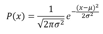
Gaussian Naive Bayes is useful when working with continuous values which probabilities can be modeled using a Gaussian distribution:

The conditional probabilities P(xi|y) are also Gaussian distributed and, therefore, it’s necessary to estimate mean and variance of each of them using the maximum likelihood approach. This quite easy, in fact, considering the property of a Gaussian, we get:

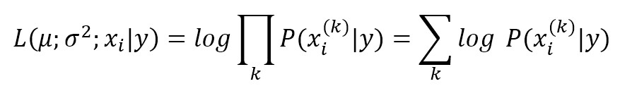
Where the k index refers to the samples in our dataset and P(xi|y) is a Gaussian itself. By minimizing the inverse of this expression (in Russel S., Norvig P., Artificial Intelligence: A Modern Approach, Pearson there’s a complete analytical explanation), we get mean and variance for each Gaussian associated to P(xi|y) and the model is hence trained.

As an example, we compare Gaussian Naive Bayes with logistic regression using the ROC curves. The dataset has 300 samples with two features. Each sample belongs to a single class:

from sklearn.datasets import make_classification

>>> nb_samples = 300
>>> X, Y = make_classification(n_samples=nb_samples, n_features=2, n_informative=2, n_redundant=0)

A plot of the dataset is shown in the following figure:

Now we can train both models and generate the ROC curves (the Y scores for naive Bayes are obtained through the predict_proba method):

from sklearn.naive_bayes import GaussianNB
from sklearn.linear_model import LogisticRegression from sklearn.metrics import roc_curve, auc
from sklearn.model_selection import train_test_split

>>> X_train, X_test, Y_train, Y_test = train_test_split(X, Y, test_size=0.25)
>>> gnb = GaussianNB()
>>> gnb.fit(X_train, Y_train)
>>> Y_gnb_score = gnb.predict_proba(X_test)
>>> lr = LogisticRegression() 
>>> lr.fit(X_train, Y_train)
>>> Y_lr_score = lr.decision_function(X_test)
>>> fpr_gnb, tpr_gnb, thresholds_gnb = roc_curve(Y_test, Y_gnb_score[:, 1])
>>> fpr_lr, tpr_lr, thresholds_lr = roc_curve(Y_test, Y_lr_score)

The resulting ROC curves are shown in the following figure:

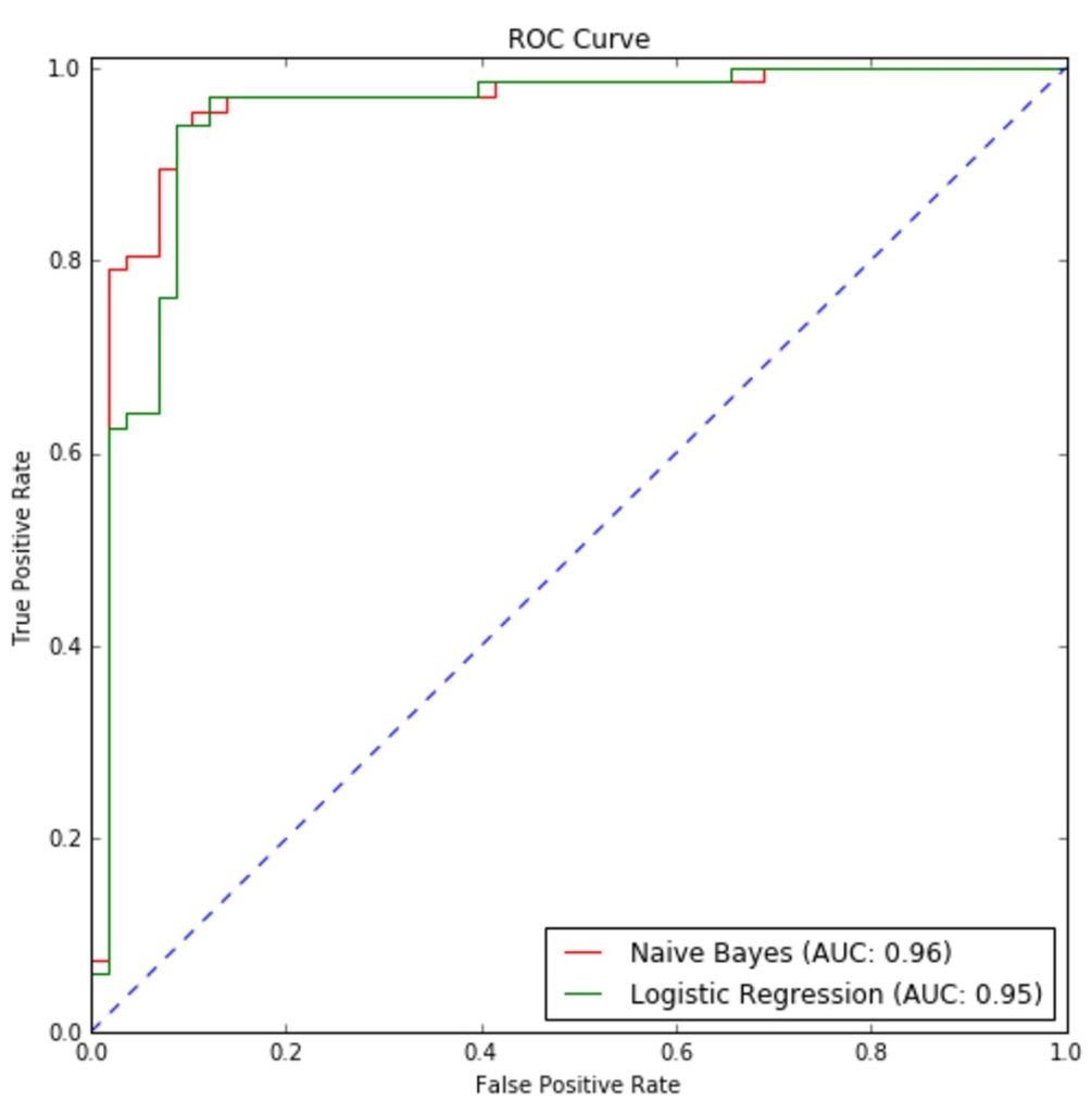
Naive Bayes performances are slightly better than logistic regression, however, the two classifiers have similar accuracy and Area Under the Curve (AUC). It’s interesting to compare the performances of Gaussian and multinomial naive Bayes with the MNIST digit dataset. Each sample (belonging to 10 classes) is an 8×8 image encoded as an unsigned integer (0 – 255), therefore, even if each feature doesn’t represent an actual count, it can be considered like a sort of magnitude or frequency.

from sklearn.datasets import load_digits
from sklearn.model_selection import cross_val_score

>>> digits = load_digits()

>>> gnb = GaussianNB()
>>> mnb = MultinomialNB()

>>> cross_val_score(gnb, digits.data, digits.target, scoring='accuracy', cv=10).mean()
0.81035375835678214

>>> cross_val_score(mnb, digits.data, digits.target, scoring='accuracy', cv=10).mean()
0.88193962163008377

The multinomial naive Bayes performs better than the Gaussian variant and the result is not really surprising. In fact, each sample can be thought as a feature vector derived from a dictionary of 64 symbols. The value can be the count of each occurrence, so a multinomial distribution can better fit the data, while a Gaussian is slightly more limited by its mean and variance.

We’ve exposed the generic naive Bayes approach starting from the Bayes’ theorem and its intrinsic philosophy. The naiveness of such algorithm is due to the choice to assume all the causes to be conditional independent. It means that each contribution is the same in every combination and the presence of a specific cause cannot alter the probability of the other ones. This is not so often realistic, however, under some assumptions; it’s possible to show that internal dependencies clear each other so that the resulting probability appears unaffected by their relations.

[box type=”note” align=”” class=”” width=””]You read an excerpt from the book, Machine Learning Algorithms, written by Giuseppe Bonaccorso. This book will help you build strong foundation to enter the world of machine learning and data science. You will learn to build a data model and see how it behaves using different ML algorithms, explore support vector machines, recommendation systems, and even create a machine learning architecture from scratch. Grab your copy today![/box]

Read Next:

What is Naïve Bayes classifier?

Machine Learning Algorithms: Implementing Naive Bayes with Spark MLlib

Implementing Apache Spark MLlib Naive Bayes to classify digital breath test data for drunk driving