


Artificial neural networks (ANN) are an abstract representation of the human nervous system, which contains a collection of neurons that communicate with each other through connections called axons. A recurrent neural network (RNN) is a class of ANN where connections between units form a directed cycle. RNNs make use of information from the past. That way, they can make predictions in data with high temporal dependencies. This creates an internal state of the network, which allows it to exhibit dynamic temporal behavior.
In this article we will look at:
- Implementation of basic RNNs in TensorFlow.
- An example of how to implement an RNN in TensorFlow for spam predictions.
- Train a model that will learn to distinguish between spam and non-spam emails using the text of the email.
This article is an extract taken from the book Deep Learning with TensorFlow – Second Edition, written by Giancarlo Zaccone, Md. Rezaul Karim.
Implementing basic RNNs in TensorFlow
TensorFlow has tf.contrib.rnn.BasicRNNCell and tf.nn.rnn_cell. BasicRNNCell, which provide the basic building blocks of RNNs. However, first let’s implement a very simple RNN model, without using either of these. The idea is to have a better understanding of what goes on under the hood.
We will create an RNN composed of a layer of five recurrent neurons using the ReLU activation function. We will assume that the RNN runs over only two-time steps, taking input vectors of size 3 at each time step. The following code builds this RNN, unrolled through two-time steps:
n_inputs = 3

n_neurons = 5

X1 = tf.placeholder(tf.float32, [None, n_inputs])

X2 = tf.placeholder(tf.float32, [None, n_inputs])

Wx = tf.get_variable("Wx", shape=[n_inputs,n_neurons], dtype=tf.

float32, initializer=None, regularizer=None, trainable=True,

collections=None)

Wy = tf.get_variable("Wy", shape=[n_neurons,n_neurons], dtype=tf.

float32, initializer=None, regularizer=None, trainable=True,

collections=None)

b = tf.get_variable("b", shape=[1,n_neurons], dtype=tf.float32,

initializer=None, regularizer=None, trainable=True, collections=None)

Y1 = tf.nn.relu(tf.matmul(X1, Wx) + b)

Y2 = tf.nn.relu(tf.matmul(Y1, Wy) + tf.matmul(X2, Wx) + b)
Then we initialize the global variables as follows:
init_op = tf.global_variables_initializer()This network looks much like a two-layer feedforward neural network, but both layers share the same weights and bias vectors. Additionally, we feed inputs at each layer and receive outputs from each layer.
X1_batch = np.array([[0, 2, 3], [2, 8, 9], [5, 3, 8], [3, 2, 9]]) # t

= 0

X2_batch = np.array([[5, 6, 8], [1, 0, 0], [8, 2, 0], [2, 3, 6]]) # t

= 1
These mini-batches contain four instances, each with an input sequence composed of exactly two inputs. At the end, Y1_val and Y2_val contain the outputs of the network at both time steps for all neurons and all instances in the mini-batch. Then we create a TensorFlow session and execute the computational graph as follows:
with tf.Session() as sess:

       init_op.run()

       Y1_val, Y2_val = sess.run([Y1, Y2], feed_dict={X1:

       X1_batch, X2: X2_batch})

Finally, we print the result:

print(Y1_val) # output at t = 0

print(Y2_val) # output at t = 1
The following is the output:
>>>

[[ 0. 0. 0. 2.56200171 1.20286 ]

[ 0. 0. 0. 12.39334488 2.7824254 ]

[ 0. 0. 0. 13.58520699 5.16213894]

[ 0. 0. 0. 9.95982838 6.20652485]]

[[ 0. 0. 0. 14.86255169 6.98305273]

[ 0. 0. 26.35326385 0.66462421 18.31009483]

[ 5.12617588 4.76199865 20.55905533 11.71787453 18.92538261]

[ 0. 0. 19.75175095 3.38827515 15.98449326]]
The network we created is simple, but if you run it over 100 time steps, for example, the graph is going to be very big.
Implementing an RNN for spam prediction
In this section, we will see how to implement an RNN in TensorFlow to predict spam/ham from texts.
Data description and preprocessing
The popular spam dataset from the UCI ML repository will be used, which can be downloaded from http://archive.ics.uci.edu/ml/machine-learning-databases/00228/smsspamcollection.zip.
The dataset contains texts from several emails, some of which were marked as spam. Here we will train a model that will learn to distinguish between spam and non-spam emails using only the text of the email. Let’s get started by importing the required libraries and model:
import os

import re

import io

import requests

import numpy as np

import matplotlib.pyplot as plt

import tensorflow as tf

from zipfile import ZipFile

from tensorflow.python.framework import ops

import warnings
Additionally, we can stop printing the warning produced by TensorFlow if you want:
warnings.filterwarnings("ignore")

os.environ['TF_CPP_MIN_LOG_LEVEL'] = '3'

ops.reset_default_graph()
Now, let’s create the TensorFlow session for the graph:
sess = tf.Session()The next task is setting the RNN parameters:
epochs = 300

batch_size = 250

max_sequence_length = 25

rnn_size = 10

embedding_size = 50

min_word_frequency = 10

learning_rate = 0.0001

dropout_keep_prob = tf.placeholder(tf.float32)
Let’s manually download the dataset and store it in a text_data.txt file in the temp directory. First, we set the path:
data_dir = 'temp'

data_file = 'text_data.txt'

if not os.path.exists(data_dir):

   os.makedirs(data_dir)
Now, we directly download the dataset in zipped format:
if not os.path.isfile(os.path.join(data_dir, data_file)):

   zip_url = 'http://archive.ics.uci.edu/ml/machine-learning-
databases/00228/smsspamcollection.zip'

   r = requests.get(zip_url)

   z = ZipFile(io.BytesIO(r.content))

   file = z.read('SMSSpamCollection')
We still need to format the data:
text_data = file.decode()

   text_data = text_data.encode('ascii',errors='ignore')

   text_data = text_data.decode().split('\n')
Now, store in it the directory mentioned earlier in a text file:
with open(os.path.join(data_dir, data_file), 'w') as
file_conn:

       for text in text_data:

           file_conn.write("{}\n".format(text))

else:

   text_data = []

   with open(os.path.join(data_dir, data_file), 'r') as
file_conn:

       for row in file_conn:

           text_data.append(row)

   text_data = text_data[:-1]
Let’s split the words that have a word length of at least 2:
text_data = [x.split('\t') for x in text_data if len(x)>=1]

[text_data_target, text_data_train] = [list(x) for x in
zip(*text_data)]
Now we create a text cleaning function:
def clean_text(text_string):

   text_string = re.sub(r'([^\s\w]|_|[0-9])+', '', text_string)

   text_string = " ".join(text_string.split())

   text_string = text_string.lower()

   return(text_string)
We call the preceding method to clean the text:
text_data_train = [clean_text(x) for x in text_data_train]Now we need to do one of the most important tasks, which is creating word embedding –changing text into numeric vectors:
vocab_processor =
tf.contrib.learn.preprocessing.VocabularyProcessor(max_sequence_length, min_frequency=min_word_frequency)

text_processed =
np.array(list(vocab_processor.fit_transform(text_data_train)))
Now let’s shuffle to make the dataset balance:
text_processed = np.array(text_processed)

text_data_target = np.array([1 if x=='ham' else 0 for x in
text_data_target])

shuffled_ix = np.random.permutation(np.arange(len(text_data_target)))

x_shuffled = text_processed[shuffled_ix]

y_shuffled = text_data_target[shuffled_ix]
Now that we have shuffled the data, we can split the data into a training and testing set:
ix_cutoff = int(len(y_shuffled)*0.75)

x_train, x_test = x_shuffled[:ix_cutoff], x_shuffled[ix_cutoff:]

y_train, y_test = y_shuffled[:ix_cutoff], y_shuffled[ix_cutoff:]

vocab_size = len(vocab_processor.vocabulary_)

print("Vocabulary size: {:d}".format(vocab_size))

print("Training set size: {:d}".format(len(y_train)))

print("Test set size: {:d}".format(len(y_test)))
Following is the output of the preceding code:
>>>

Vocabulary size: 933

Training set size: 4180

Test set size: 1394
Before we start training, let’s create placeholders for our TensorFlow graph:
x_data = tf.placeholder(tf.int32, [None, max_sequence_length])

y_output = tf.placeholder(tf.int32, [None])
Let’s create the embedding:
embedding_mat = tf.get_variable("embedding_mat",
shape=[vocab_size, embedding_size], dtype=tf.float32,
initializer=None, regularizer=None, trainable=True, collections=None)

embedding_output = tf.nn.embedding_lookup(embedding_mat, x_data)
Now it’s time to construct our RNN. The following code defines the RNN cell:
cell = tf.nn.rnn_cell.BasicRNNCell(num_units = rnn_size)

output, state = tf.nn.dynamic_rnn(cell, embedding_output,
dtype=tf.float32)

output = tf.nn.dropout(output, dropout_keep_prob)
Now let’s define the way to get the output from our RNN sequence:
output = tf.transpose(output, [1, 0, 2])

last = tf.gather(output, int(output.get_shape()[0]) - 1)
Next, we define the weights and the biases for the RNN:
weight = bias = tf.get_variable("weight", shape=[rnn_size, 2],
dtype=tf.float32, initializer=None, regularizer=None,
trainable=True, collections=None)

bias = tf.get_variable("bias", shape=[2], dtype=tf.float32,
initializer=None, regularizer=None, trainable=True,
collections=None)
The logits output is then defined. It uses both the weight and the bias from the preceding code:
logits_out = tf.nn.softmax(tf.matmul(last, weight) + bias)

Now we define the losses for each prediction so that later on, they can contribute to the loss function:

losses =
tf.nn.sparse_softmax_cross_entropy_with_logits_v2(logits=logits_ou
t, labels=y_output)
We then define the loss function:
loss = tf.reduce_mean(losses)We now define the accuracy of each prediction:
accuracy = tf.reduce_mean(tf.cast(tf.equal(tf.argmax(logits_out, 1), tf.cast(y_output, tf.int64)), tf.float32))We then create the training_op with RMSPropOptimizer:
optimizer = tf.train.RMSPropOptimizer(learning_rate)

train_step = optimizer.minimize(loss)
Now let’s initialize all the variables using the global_variables_initializer() method:
init_op = tf.global_variables_initializer()

sess.run(init_op)
Additionally, we can create some empty lists to keep track of the training loss, testing loss, training accuracy, and the testing accuracy in each epoch:
train_loss = []

test_loss = []

train_accuracy = []

test_accuracy = []
Now we are ready to perform the training, so let’s get started. The workflow of the training goes as follows:
- Shuffle the training data
- Select the training set and calculate generations
- Run training step for each batch
- Run loss and accuracy of training
- Run the evaluation steps.
The following codes include all of the aforementioned steps:
shuffled_ix = np.random.permutation(np.arange(len(x_train)))

   x_train = x_train[shuffled_ix]

   y_train = y_train[shuffled_ix]

   num_batches = int(len(x_train)/batch_size) + 1


   for i in range(num_batches):

       min_ix = i * batch_size

       max_ix = np.min([len(x_train), ((i+1) * batch_size)])

       x_train_batch = x_train[min_ix:max_ix]

       y_train_batch = y_train[min_ix:max_ix]

       train_dict = {x_data: x_train_batch, y_output: \

y_train_batch, dropout_keep_prob:0.5}

       sess.run(train_step, feed_dict=train_dict)

       temp_train_loss, temp_train_acc = sess.run([loss,\

                        accuracy], feed_dict=train_dict)

   train_loss.append(temp_train_loss)

   train_accuracy.append(temp_train_acc)

   test_dict = {x_data: x_test, y_output: y_test, \

dropout_keep_prob:1.0}

   temp_test_loss, temp_test_acc = sess.run([loss, accuracy], \

                   feed_dict=test_dict)

   test_loss.append(temp_test_loss)

   test_accuracy.append(temp_test_acc)

   print('Epoch: {}, Test Loss: {:.2}, Test Acc: {:.2}'.format(epoch+1, temp_test_loss, temp_test_acc))

print('\nOverall accuracy on test set (%):
{}'.format(np.mean(temp_test_acc)*100.0))
Following is the output of the preceding code:
>>>

Epoch: 1, Test Loss: 0.68, Test Acc: 0.82

Epoch: 2, Test Loss: 0.68, Test Acc: 0.82

Epoch: 3, Test Loss: 0.67, Test Acc: 0.82

…

Epoch: 997, Test Loss: 0.36, Test Acc: 0.96

Epoch: 998, Test Loss: 0.36, Test Acc: 0.96

Epoch: 999, Test Loss: 0.35, Test Acc: 0.96

Epoch: 1000, Test Loss: 0.35, Test Acc: 0.96

Overall accuracy on test set (%): 96.19799256324768
Well done! The accuracy of the RNN is above 96%, which is outstanding. Now let’s observe how the loss propagates across each iteration and over time:
epoch_seq = np.arange(1, epochs+1)

plt.plot(epoch_seq, train_loss, 'k--', label='Train Set')

plt.plot(epoch_seq, test_loss, 'r-', label='Test Set')

plt.title('RNN training/test loss')

plt.xlabel('Epochs')

plt.ylabel('Loss')

plt.legend(loc='upper left')

plt.show()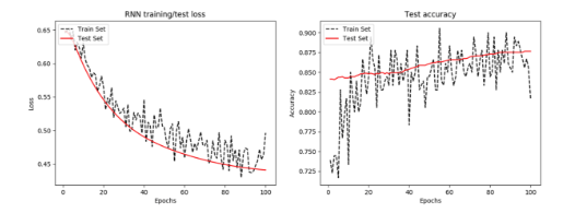
Figure 1: a) RNN training and test loss per epoch b) test accuracy per epoch
We also plot the accuracy over time:
plt.plot(epoch_seq, train_accuracy, 'k--', label='Train Set')

plt.plot(epoch_seq, test_accuracy, 'r-', label='Test Set')

plt.title('Test accuracy')

plt.xlabel('Epochs')

plt.ylabel('Accuracy')

plt.legend(loc='upper left')

plt.show()
We discussed the implementation of RNNs in TensorFlow. We saw how to make predictions with data that has a high temporal dependency and how to develop real-life predictive models that make the predictive analytics easier using RNNs. If you want to delve into neural networks and implement deep learning algorithms check out this book, Deep learning with TensorFlow – Second Edition.
Read Next:
Top 5 Deep Learning Architectures


