How to Denoise Images with Neural Networks

The premise of denoising images is very useful and can be applied to images, sounds, texts, and more. While deep learning is possibly not the best approach, it is an interesting one, and shows how versatile deep learning can be.

Get The Data

The data we will be using is a dataset of faces from github user hromi. It’s a fun dataset to play around with because it has both smiling and non-smiling images of faces and it’s good for a lot of different scenarios, such as training to find a smile or training to fill missing parts of images.

The data is neatly packaged in a zip and is easily accessed with the following:

import os
import numpy as np
import zipfile
from urllib import request
import matplotlib.pyplot as plt
import matplotlib.image as mpimg
import random
%matplotlib inline

url = 'https://github.com/hromi/SMILEsmileD/archive/master.zip'
request.urlretrieve(url, 'data.zip')
zipfile.ZipFile('data.zip').extractall()

This will download all of the images to a folder with a variety of peripheral information we will not be using, but would be incredibly fun to incorporate into a model in other ways.

Preview images

First, let’s load all of the data and preview some images:

x_pos = []
base_path = 'SMILEsmileD-master/SMILEs/'
positive_smiles = base_path + 'positives/positives7/'
negative_smiles = base_path + 'SMILEsmileD-master/SMILEs/negatives/negatives7/'
for img in os.listdir(positive_smiles):
    x_pos.append(mpimg.imread(positive_smiles + img))
# change into np.array and scale to 255. which is max
x_pos = np.array(x_pos)/255.
# reshape which is explained later
x_pos = x_pos.reshape(len(x_pos),1,64,64)

# plot 3 random images
plt.figure(figsize=(8, 6))
n = 3
for i in range(n):
    ax = plt.subplot(2, 3, i+1) # using i+1 since 0 is deprecated in future matplotlib
    plt.imshow(random.choice(x_pos), cmap=plt.cm.gray)
    ax.get_xaxis().set_visible(False)
    ax.get_yaxis().set_visible(False)

Below is what you should get:

Visualize Noise

From here let’s add a random amount of noise and visualize it.

plt.figure(figsize=(8, 10))
plt.subplot(3,2,1).set_title('normal')
plt.subplot(3,2,2).set_title('noisy')
plt.tight_layout()
n = 6
for i in range(1,n+1,2):
    # 2 columns with good on left side, noisy on right side
    ax = plt.subplot(3, 2, i)

    rand_img = random.choice(x_pos)[0]
    random_factor = 0.05 * np.random.normal(loc=0., scale=1., size=rand_img.shape)
    # plot normal images
    plt.imshow(rand_img, cmap=plt.cm.gray)
    ax.get_xaxis().set_visible(False)
    ax.get_yaxis().set_visible(False)
    # plot noisy images
    ax = plt.subplot(3,2,i+1)

    plt.imshow(rand_img + random_factor, cmap=plt.cm.gray)
    ax.get_yaxis().set_visible(False)
    ax.get_xaxis().set_visible(False)

Below is comparison of normal image on the left and a noisy image on the right:

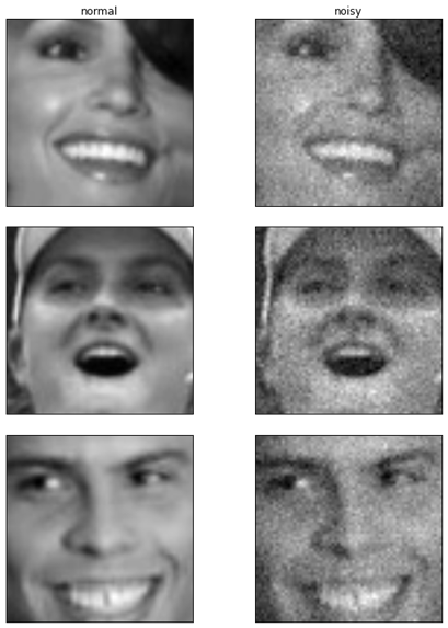
As you can see, the images are still visually similar to the normal images but this technique can be very useful if an image is blurry or very grainy due to the high ISO in traditional cameras.

Prepare the Dataset

From here it’s always good practice to split the dataset if we intend to evaluate our model later, so we will split the data into a train and a test set. We will also shuffle the images, since I am unaware of any requirement for order to the data.

# shuffle the images in case there was some underlying order
np.random.shuffle(x_pos)
# split into test and train set, but we will use keras built in validation_size
x_pos_train = x_pos[int(x_pos.shape[0]* .20):]
x_pos_test = x_pos[:int(x_pos.shape[0]* .20)]
x_pos_noisy = x_pos_train + 0.05 * np.random.normal(loc=0., scale=1., size=x_pos_train.shape)

Training Model

The model we are using is based off of the new Keras functional API with a Sequential comparison as well.

Quick intro to Keras Functional API

While previously there was the graph and sequential model, almost all models used the Sequential form. This is the standard type of modeling in deep learning and consists of a linear ordering of layer to layer (that is, no merges or splits).

Using the Sequential model is the same as before and is incredibly modular and understandable since the model is composed by adding layer upon layer. For example, our keras model in Sequential form will look like the following:

from keras.models import Sequential
from keras.layers import Dense, Activation, Convolution2D, MaxPooling2D, UpSampling2D


seqmodel = Sequential()
seqmodel.add(Convolution2D(32, 3, 3, border_mode='same', input_shape=(1, 64,64)))
seqmodel.add(Activation('relu'))
seqmodel.add(MaxPooling2D((2, 2), border_mode='same')

seqmodel.add(Convolution2D(32, 3, 3, border_mode='same'))
seqmodel.add(Activation('relu'))
seqmodel.add(UpSampling2D((2, 2))
seqmodel.add(Convolution2D(1, 3, 3, border_mode='same'))
seqmodel.add(Activation('sigmoid'))

seqmodel.compile(optimizer='adadelta', loss='binary_crossentropy')

Versus the Functional Model format:

from keras.layers import Input, Dense, Convolution2D, MaxPooling2D, UpSampling2D
from keras.models import Model

input_img = Input(shape=(1, 64, 64))
x = Convolution2D(32, 3, 3, border_mode='same')(input_img)
x = Activation('relu')(x)
x = MaxPooling2D((2, 2), border_mode='same')(x)

x = Convolution2D(32, 3, 3, border_mode='same')(x)
x = Activation('relu')(x)
x = UpSampling2D((2, 2))(x)
x = Convolution2D(1, 3, 3, activation='sigmoid', border_mode='same')(x)

funcmodel = Model(input_img, x)
funcmodel.compile(optimizer='adadelta', loss='binary_crossentropy')

While these models look very similar, the functional form is more versatile at the cost of being more confusing.

Let’s fit these and compare the results to show that they are equivalent:

seqmodel.fit(x_pos_noisy,
             x_pos_train,
             nb_epoch=10,
             batch_size=32,
             shuffle=True,
             validation_split=.20)


funcmodel.fit(x_pos_noisy,
              x_pos_train,
              nb_epoch=10,
              batch_size=32,
              shuffle=True,
              validation_split=.20)

Following the training time and loss functions should net near-identical results. For the sake of argument, we will plot outputs from both models and show how they result in near identical results.

# create noisy test set and create predictions from sequential and function
x_noisy_test = x_pos_test + 0.05 * np.random.normal(loc=0., scale=1., size=x_pos_test.shape)
f1 = funcmodel.predict(x_noisy_test)
s1 = seqmodel.predict(x_noisy_test)


plt.figure(figsize=(12, 12))
plt.subplot(3,4,1).set_title('normal')
plt.subplot(3,4,2).set_title('noisy')
plt.subplot(3,4,3).set_title('denoised-functional')
plt.subplot(3,4,4).set_title('denoised-sequential')
n = 3
for i in range(1,12,4):
    img_index = random.randint(0,len(x_noisy_test))
    # plot original image
    ax = plt.subplot(3, 4, i)
    plt.imshow(x_pos_test[img_index][0], cmap=plt.cm.gray)
    ax.get_xaxis().set_visible(False)
    ax.get_yaxis().set_visible(False)

    # plot noisy images
    ax = plt.subplot(3,4,i+1)
    plt.imshow(x_noisy_test[img_index][0], cmap=plt.cm.gray)
    ax.get_yaxis().set_visible(False)
    ax.get_xaxis().set_visible(False)

    # plot denoised functional
    ax = plt.subplot(3,4,i+2)
    plt.imshow(f1[img_index][0], cmap=plt.cm.gray)
    ax.get_yaxis().set_visible(False)
    ax.get_xaxis().set_visible(False)

    # plot denoised sequential
    ax = plt.subplot(3,4,i+3)
    plt.imshow(s1[img_index][0], cmap=plt.cm.gray)
    ax.get_yaxis().set_visible(False)
    ax.get_xaxis().set_visible(False)
plt.tight_layout()

The result will be something like this.

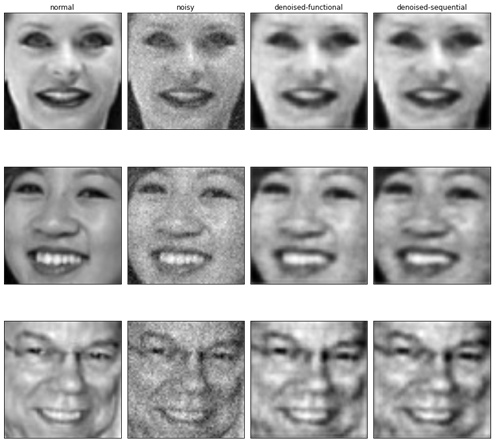
Since we only trained the net with 10 epochs and it was very shallow, we also could add more layers, use more epochs, and see if it nets in better results:

seqmodel = Sequential()
seqmodel.add(Convolution2D(32, 3, 3, border_mode='same', input_shape=(1, 64,64)))
seqmodel.add(Activation('relu'))
seqmodel.add(MaxPooling2D((2, 2), border_mode='same'))

seqmodel.add(Convolution2D(32, 3, 3, border_mode='same'))
seqmodel.add(Activation('relu'))
seqmodel.add(MaxPooling2D((2, 2), border_mode='same'))

seqmodel.add(Convolution2D(32, 3, 3, border_mode='same'))
seqmodel.add(Activation('relu'))
seqmodel.add(UpSampling2D((2, 2)))

seqmodel.add(Convolution2D(32, 3, 3, border_mode='same'))
seqmodel.add(Activation('relu'))
seqmodel.add(UpSampling2D((2, 2)))

seqmodel.add(Convolution2D(1, 3, 3, border_mode='same'))
seqmodel.add(Activation('sigmoid'))
seqmodel.compile(optimizer='adadelta', loss='binary_crossentropy')

seqmodel.fit(x_pos_noisy,
             x_pos_train,
             nb_epoch=50,
             batch_size=32,
             shuffle=True,
             validation_split=.20,
             verbose=0)
s2 = seqmodel.predict(x_noisy_test)
plt.figure(figsize=(10, 10))
plt.subplot(3,3,1).set_title('normal')
plt.subplot(3,3,2).set_title('noisy')
plt.subplot(3,3,3).set_title('denoised')
for i in range(1,9,3):
    img_index = random.randint(0,len(x_noisy_test))
    # plot original image
    ax = plt.subplot(3, 3, i)
    plt.imshow(x_pos_test[img_index][0], cmap=plt.cm.gray)
    ax.get_xaxis().set_visible(False)
    ax.get_yaxis().set_visible(False)

    # plot noisy images
    ax = plt.subplot(3,3,i+1)
    plt.imshow(x_noisy_test[img_index][0], cmap=plt.cm.gray)
    ax.get_yaxis().set_visible(False)
    ax.get_xaxis().set_visible(False)

    # plot denoised functional
    ax = plt.subplot(3,3,i+2)
    plt.imshow(s2[img_index][0], cmap=plt.cm.gray)
    ax.get_yaxis().set_visible(False)
    ax.get_xaxis().set_visible(False)

plt.tight_layout()

While this is a small example, it’s easily extendable to other scenarios. The ability to denoise an image is by no means new and unique to neural networks, but is an interesting experiment about one of the many uses that show potential for deep learning.

About the author

Graham Annett is an NLP Engineer at Kip (Kipthis.com).  He has been interested in deep learning for a bit over a year and has worked with and contributed to Keras.  He can be found on GitHub or via here .