


Chainer is a powerful, flexible, and intuitive framework for deep learning. In this post, I will help you to get started with Chainer.
Why is Chainer important to learn? With its “Define by run” approach, it provides very flexible and easy ways to construct—and debug if you encounter some troubles—network models. It also works efficiently with well-tuned numpy. Additionally, it provides transparent GPU access facility with a fairly sophisticated cupy library, and it is actively developed.
How to install Chainer
Here I’ll show you how to install Chainer. Chainer has CUDA and cuDNN support. If you want to use Chainer with them, follow along in the “Install Chainer with CUDA and cuDNN support” section.
Install Chainer via pip
You can install Chainer easily via pip, which is the officially recommended way.
$ pip install chainerInstall Chainer from source code
You can also install it from its source code.
$ tar zxf chainer-x.x.x.tar.gz
$ cd chainer-x.x.x
$ python setup.py install
Install Chainer with CUDA and cuDNN support
Chainer has GPU support with Nvidia CUDA. If you want to use Chainer with CUDA support, install the related software in the following order.
- Install CUDA Toolkit
- (optional) Install cuDNN
- Install Chainer
Chainer has cuDNN suport as well as CUDA. cuDNN is a library for accelerating deep neural networks and Nvidia provides it. If you want to enable cuDNN support, install cuDNN in an appropriate path before installing Chainer. The recommended install path is in the CUDA Toolkit directory.
$ cp /path/to/cudnn.h $CUDA_PATH/include
$ cp /path/to/libcudnn.so* $CUDA_PATH/lib64
After that, if the CUDA Toolkit (and cuDNN if you want) is installed in its default path, the Chainer installer finds them automatically.
$ pip install chainerIf CUDA Toolkit is in a directory other than the default one, setting the CUDA_PATH environment variable helps.
$ CUDA_PATH=/opt/nvidia/cuda pip install chainerIn case you have already installed Chainer before setting up CUDA (and cuDNN), reinstall Chainer after setting them up.
$ pip uninstall chainer
$ pip install chainer --no-cache-dir
Trouble shooting
If you have some trouble installing Chainer, using the -vvvv option with the pip command may help you. It shows all logs during installation.
$ pip install chainer -vvvvTrain multi-layer perceptron with MNIST dataset
Now I cover how to train the multi-layer perceptron (MLP) model with the MNIST handwritten digit dataset with Chainer is shown. It is very simple because Chainer provides an example program to do it. Additionally, we run the program on GPU to compare its training efficiency between CPU and GPU.
Run MNIST example program
Chainer proves an example program to train the multi-layer perceptron (MLP) model with the MNIST dataset.
$ cd chainer/examples/mnist
$ ls *.py
data.py net.py train_mnist.pydata.py, which is used from train_mnist.py, is a script for downloading the MNIST dataset from the Internet. net.py is also used from train_mnist.py as a script where a MLP network model is defined.
train_mnist.py is a script we run to train the MLP model. It does the following things:
- Download and convert the MNIST dataset.
- Prepare an MLP model.
- Train the MLP model with the MNIST dataset.
- Test the trained MLP model.
Here we run the train_mnist.py script on the CPU. It may take a couple of hours depending on your machine spec.
$ python train_mnist.py
GPU: -1
# unit: 1000
# Minibatch-size: 100
# epoch: 20
Network type: simple

load MNIST dataset
Downloading train-images-idx3-ubyte.gz...
Done
Downloading train-labels-idx1-ubyte.gz...
Done
Downloading t10k-images-idx3-ubyte.gz...
Done
Downloading t10k-labels-idx1-ubyte.gz...
Done
Converting training data...
Done
Converting test data...
Done
Save output...
Done
Convert completed
epoch 1
graph generated
train mean loss=0.192189417146, accuracy=0.941533335938, throughput=121.97765842 images/sec
test mean loss=0.108210202637, accuracy=0.966000005007
epoch 2
train mean loss=0.0734026790201, accuracy=0.977350010276, throughput=122.715585263 images/sec
test mean loss=0.0777539889357, accuracy=0.974500003457
...
epoch 20
train mean loss=0.00832913763473, accuracy=0.997666668793, throughput=121.496046895 images/sec
test mean loss=0.131264564424, accuracy=0.978300007582
save the model
save the optimizer
After training for 20 epochs, the MLP model is well trained to achieve a loss value of around 0.131 and accuracy of around 0.978 in testing. The trained model and state files are stored as mlp.model and mlp.state respectively, so we can resume training or testing with them.
Accelerate training MLP with GPU
The train_mnist.py script has a –gpu option to train the MLP model on GPU. To use it, specify which GPU you use giving a GPU index that is an integer beginning from 0. -1 means you are using CPU.
$ python train_mnist.py --gpu 0
GPU: 0
# unit: 1000
# Minibatch-size: 100
# epoch: 20
Network type: simple

load MNIST dataset
epoch 1
graph generated
train mean loss=0.189480076165, accuracy=0.942750002556, throughput=12713.8872884 images/sec
test mean loss=0.0917134844698, accuracy=0.97090000689
epoch 2
train mean loss=0.0744868403107, accuracy=0.976266676188, throughput=14545.6445472 images/sec
test mean loss=0.0737037020434, accuracy=0.976600006223
...
epoch 20
train mean loss=0.00728972356146, accuracy=0.9978333353, throughput=14483.9658281 images/sec
test mean loss=0.0995463995047, accuracy=0.982400006056
save the model
save the optimizer
After training for 20 epochs, the MLP model is trained as well as on CPU to get a loss value of around 0.0995 and accuracy of around 0.982 in testing.
Compared in average throughput, the GPU is more than 10,000 images/sec than that on CPU, shown in the previous section at around 100 images/sec[VP1] . While the CPU of my machine is a bit too poor compared with its GPU, in fairness the CPU version runs in a single thread, but this result should be enough to illustrate the efficiency of training on the GPU.
Little code required to run Chainer on GPU
The code required to run Chainer on GPU is less. In the train_mnist.py script, only the three treatments are needed:
- Select the GPU device to use.
- Transfer the network model to GPU.
- Allocate the multi-dimensional matrix on the GPU device installed on the host.
The following lines are related to train_mnist.py.
...
if args.gpu >= 0:
   cuda.get_device(args.gpu).use()
   model.to_gpu()
xp = np if args.gpu < 0else cuda.cupy
...
and
...
for i in six.moves.range(0, N, batchsize):
   x = chainer.Variable(xp.asarray(x_train[perm[i:i + batchsize]]))
   t = chainer.Variable(xp.asarray(y_train[perm[i:i + batchsize]]))
...
Run Caffe reference models on Chainer
Chainer has a powerful feature to interpret pre-trained Caffe reference models. This makes us able to use those models easily on Chainer without enormous training efforts. In this part we import the pre-trained GoogLeNet model and use it to predict what an input image means.
Model Zoo directory
Chainer has a Model Zoo directory in the following path.
$ cd chainer/example/modelzooDownload Caffe reference model
First, download a Caffe reference model from BVLC Model Zoo. Chainer provides a simple script for that. This time use the pre-trained GoogLeNet model.
$ python download_model.py googlenet
Downloading model file...
Done
$ ls *.caffemodel
bvlc_googlenet.caffemodel
Download ILSVRC12 mean file
We also download the ILSVRC12 mean image file, which Chainer uses. This mean image is used to subtract from images we want to predict.
$ python download_mean_file.py
Downloading ILSVRC12 mean file for NumPy...
Done
$ ls *.npy
ilsvrc_2012_mean.npy
Get ILSVRC12 label descriptions
Because the output of the Caffe reference model is a set of label indices as integers, we cannot find out which index means which category of images. So we get label descriptions from BVLC. The row numbers correspond to the label indices of the model.
$ wget -c http://dl.caffe.berkeleyvision.org/caffe_ilsvrc12.tar.gz
$ tar -xf caffe_ilsvrc12.tar.gz
$ cat synset_words.txt | awk '{$1=""; print}' > labels.txt
$ cat labels.txt
tench, Tinca tinca
goldfish, Carassius auratus
great white shark, white shark, man-eater, man-eating shark, Carcharodon carcharias
tiger shark, Galeocerdo cuvieri
hammerhead, hammerhead shark
electric ray, crampfish, numbfish, torpedo
stingray
cock
hen
ostrich, Struthio camelus
...
Mac OS X does not have a wget command, so you can use the curl command instead.
$ curl -O http://dl.caffe.berkeleyvision.org/caffe_ilsvrc12.tar.gzPython script to run Caffe reference model
While there is an evaluate_caffe_net.py script in the modelzoo directory, it is for evaluating the accuracy of interpreted Caffe reference models against the ILSVRC12 dataset. Now input an image and predict what it means. So use another predict_caffe_net.py script that is not included in the modelzoo directory. Here is that code listing.
#!/usr/bin/env python

from __future__ import print_function
import argparse
import sys

import numpy as np
from PIL import Image

import chainer
import chainer.functions as F
from chainer.links import caffe

in_size = 224

# Parse command line arguments.
parser = argparse.ArgumentParser()
parser.add_argument('image', help='Path to input image file.')
parser.add_argument('model', help='Path to pretrained GoogLeNet Caffe model.')
args = parser.parse_args()

# Constant mean over spatial pixels.
mean_image = np.ndarray((3, in_size, in_size), dtype=np.float32)
mean_image[0] = 104
mean_image[1] = 117
mean_image[2] = 123

# Prepare input image.
def resize(image, base_size):
   width, height = image.size
   if width > height:
       new_width = base_size * width / height
       new_height = base_size
   else:
       new_width = base_size
       new_height = base_size * height / width
   return image.copy().resize((new_width, new_height))

def clip_center(image, size):
   width, height = image.size
   width_offset = (width - size) / 2
   height_offset = (height - size) / 2
   box = (width_offset, height_offset,
           width_offset + size, height_offset + size)
   image1 = image.crop(box)
   image1.load()
   return image1

image = Image.open(args.image)
image = resize(image, 256)
image = clip_center(image, in_size)
image = np.asarray(image).transpose(2, 0, 1).astype(np.float32)
image -= mean_image

# Make input data from the image.
x_data = np.ndarray((1, 3, in_size, in_size), dtype=np.float32)
x_data[0] = image

# Load Caffe model file.
print('Loading Caffe model file ...', file=sys.stderr)
func = caffe.CaffeFunction(args.model)
print('Loaded', file=sys.stderr)

# Predict input image.
def predict(x):
   y, = func(inputs={'data': x}, outputs=['loss3/classifier'],
             disable=['loss1/ave_pool', 'loss2/ave_pool'],
             train=False)
   return F.softmax(y)

x = chainer.Variable(x_data, volatile=True)
y = predict(x)

# Print prediction scores.
categories = np.loadtxt("labels.txt", str, delimiter="t")
top_k = 20
result = zip(y.data[0].tolist(), categories)
result.sort(cmp=lambda x, y: cmp(x[0], y[0]), reverse=True)
for rank, (score, name) in enumerate(result[:top_k], start=1):
   print('#%d | %4.1f%% | %s' % (rank, score * 100, name))
You may need to install Pillow to run this script. Pillow is a Python imaging library and we use it to manipulate input images.
$ pip install pillowRun Caffe reference model
Now you can run the pre-trained GoogLeNet model on Chainer for prediction. This time, we use the following JPEG image of a dog, specially classified as a long coat Chihuahua in dog breeds.
$ ls *.jpg
image.jpg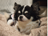 Sample image
To predict, just run the predict_caffe_net.py script.
$ python predict_caffe_net.py image.jpg googlenet bvlc_googlenet.caffemodel
Loading Caffe model file bvlc_googlenet.caffemodel...
Loaded
#1 | 48.2% | Chihuahua
#2 | 24.5% | Japanese spaniel
#3 | 24.2% | papillon
#4 | 1.1% | Pekinese, Pekingese, Peke
#5 | 0.5% | Boston bull, Boston terrier
#6 | 0.4% | toy terrier
#7 | 0.2% | Border collie
#8 | 0.2% | Pomeranian
#9 | 0.1% | Shih-Tzu
#10 | 0.1% | bow tie, bow-tie, bowtie
#11 | 0.0% | feather boa, boa
#12 | 0.0% | tennis ball
#13 | 0.0% | Brabancon griffon
#14 | 0.0% | Blenheim spaniel
#15 | 0.0% | collie
#16 | 0.0% | quill, quill pen
#17 | 0.0% | sunglasses, dark glasses, shades
#18 | 0.0% | muzzle
#19 | 0.0% | Yorkshire terrier
#20 | 0.0% | sunglass
Here GoogLeNet predicts that most likely the input image means Chihuahua, which is the correct answer.
While its prediction percentage is 48.2%, the following candidates are Japanese spaniel (aka. Japanese Chin) and papillon, which are hard to distinguish from Chihuahua even for human eyes at a glance.
Conclusion
In this post, I showed you some basic entry points to start using Chainer. The first is how to install Chainer. Then we saw how to train a multi-layer perceptron with the MNIST dataset on Chainer, illustrating the efficiency of training on GPU, which you can get easily on Chainer. Finally, I indicated how to run the Caffe reference model on Chainer, which enables you to use pre-trained Caffe models out of the box.
As next steps, you may want to learn:
- Playing with other Chainer examples.
- Defining your own network models.
- Implementing your own functions.
For details, Chainer’s official documentation will help you.
About the author
Masayuki Takagi is an entrepreneur and software engineer from Japan. His professional experience domains are advertising and deep learning, serving big Japanese corporations. His personal interests are fluid simulation, GPU computing, FPGA, and compiler and programming language design. Common Lisp is his most beloved programming language and he is the author of the cl-cuda library. Masayuki is a graduate of the university of Tokyo and lives in Tokyo with his buddy Plum, a long coat Chihuahua, and aco.


