Getting started with the Jupyter notebook (part 2)

As seen in the first part of this introduction, you can do a lot of things with the basic capabilities of the Jupyter notebook. But it offers even more possibilities and options, allowing users to create beautiful, interactive documents.

Cells manipulation

When writing your notebook, you will want to use more advanced cell manipulation. Thankfully, the notebook allows you to manipulate a variety of operations on your cells. You can delete a cell by selecting the desired cell, then going to Edit -> Delete cell, you can move cells by going to Edit -> Move cell [up | down], or you can cut the cell and paste it by going Edit -> Cut Cell then Edit -> Paste Cell …, selecting the pasting style you need. You can also merge cells, by going to Edit -> Merge cell [above|below], if you find that you have so many cells that you execute only once, or if you want a big chunk of code to be executed in a single sweep. Keep these commands in mind when writing your notebook — they will save you a lot of time.

Markdown cells advanced usage

Let’s start by exploring the markdown cell type a little more. Even though it says markdown, this type of cell also accepts HTML code. Using this, you can create more advanced styling within your cell, add images and so on. For example, if you want to add the Jupyter logo to your notebook, with a size of 100px by 100px, on the left of the cell:

<img src="http://blog.jupyter.org/content/images/2015/02/jupyter-sq-text.png"
style="width:100px;height:100px;float:left">

This provides the following after the cell evaluation:

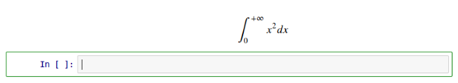
Let’s end with the capabilities of the markdown cells: they also support LaTeX syntax. Write your equations in a markdown cell, evaluate the cell, and look at the result. By evaluating this equation:

$$int_0^{+infty} x^2 dx$$

You get the LaTeX equation:

Export capabilities

Another powerful feature of the notebook is the export capability. Indeed, you can write your notebook (an illustrated coding course, for example) and export it in multiple formats such as:

• HTML
• Markdown
• ReST
• PDF (Through LaTeX)
• Raw Python

By exporting to PDF, you can then create a beautiful document using LaTeX without even using LaTeX! Or you can publish your notebook as a page on your personnal website. You can even write documentation for libraries by exporting to ReST.

Matplotlib integration

If you have ever done plotting using Python, then you probably know about matplotlib. Matplotlib is a Python library used to create beautiful plots. And it really shines when used with the Jupyter notebook. Let’s start exploring what can be done with it.

To get started using matplotlib in the Jupyter notebook, you need to tell Jupyter to get all images generated by matplotlib and include them in the notebook. To do that, you just evaluate:

%matplotlib inline

It might take a few seconds to run, but you only need to do this once when you start your notebook. Let’s make a plot and see how this integration works:

import matplotlib.pyplot as plt
import numpy as np

x = np.arange(20)
y = x**2

plt.plot(x, y)

This simple code will just plot the equation y=x^2. When you evaluate the cell, you get:

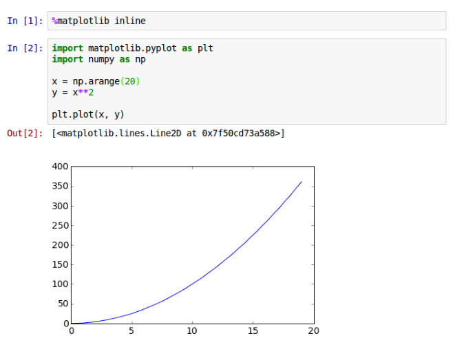
As you can see here, the plot was added directly into the notebook, just after the code. We can then change our code, reevaluate, and the image will be updated on the fly. This is a nice feature for every data scientist wanting to have their code and images in the same file, letting them know which code does what exactly. Being able to add some more text to the document is also a great help.

Non local kernel

The Jupyter notebook is built in such a way that it is very easy to start Jupyter from a computer, and allow multiple people to connect to the same Jupyter instance through network. Did you notice, in the previous part of this introduction, the following sentence during Jupyter startup:

The IPython Notebook is running at: http://localhost:8888/

This means that your notebook is running locally, on your computer, and that you can access it through a browser at the address http://localhost:8888/. It is possible to make the notebook publicly available by changing the configuration. This will allow anyone with the address to connect to this notebook and make modifications to the notebooks remotely, through their Internet browser.

The end word

As we have seen in these two parts, the Jupyter notebook is a very powerful tool, allowing users to create beautiful documents for data exploration, education, documentation, and, actually, everything you can think of. Don’t hesitate to explore more of its possibilities, and give feedback to the developers if you ever run into trouble, or even if you just want to thank them.

About the author

Marin Gilles is a PhD student in Physics in Dijon, France. A large part of his work is dedicated to physical simulations for which he developed his own simulation framework using Python, and contributed to open-source libraries such as Matplotlib or IPython.