


The Jupyter notebook (previously known as IPython notebooks) is an interactive notebook, in which you can run code from more than 40 programming languages. In this introduction, we will explore the main features of the Jupyter notebook and see why it can be such a poweful tool for anyone wanting to create beautiful interactive documents and educational resources.
To start this working with the notebook, you will need to install it. You can find the full procedure on the Jupyter website.
jupyter notebookYou will see something similar to the following displayed :
[I 20:06:36.367 NotebookApp] Writing notebook server cookie secret to /run/user/1000/jupyter/notebook_cookie_secret
[I 20:06:36.813 NotebookApp] Serving notebooks from local directory: /home/your_username
[I 20:06:36.813 NotebookApp] 0 active kernels
[I 20:06:36.813 NotebookApp] The IPython Notebook is running at: http://localhost:8888/
[I 20:06:36.813 NotebookApp] Use Control-C to stop this server and shut down all kernels (twice to skip confirmation).
And the main Jupyter window should open in the folder you started the notebook (usually your user folder). The main window looks like this :
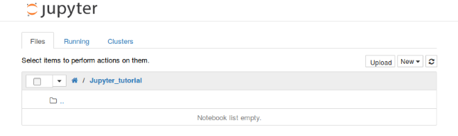
To create a new notebook, simply click on New and choose the kind of notebook you wish to start under the notebooks section.
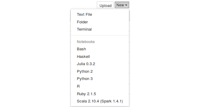
I only have a Python kernel installed locally, so I will start a Python notebook to start working with. A new tab opens, and I get the notebook interface, completely empty.
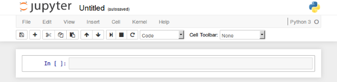
You can see different parts of the notebook:
- Name of your notebook
- Main toolbar, with options to save your notebook, export, reload, un notebook[RB1] , restart kernel, etc.
- Shortcuts
- The main part of the notebook, containing the contents of your notebook
Take the time to explore the menus and see your options. If you need help on a very specific subject, concerning the notebook or some libraries, you can try the help menu at the right end of the menu bar.
In the main area, you can see what is called a cell. Each notebook is composed of multiple cells, and each cell will be used for a different purpose.
The first cell we have here, starting with In [ ] is a code cell. In this type of cell, you can type any code and execute it. For example, try typing 1 + 2 then hit Shift + Enter. When hitting Shift + Enter, the code in the cell will be evaluated, you will be placed in a new cell, and you will get the following:
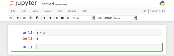
You can easily identify the current working cell thanks to the green outline. Let’s type something else in the second cell, for example:
for i in range(5):
    print(i)
When evaluating this cell, you then get:
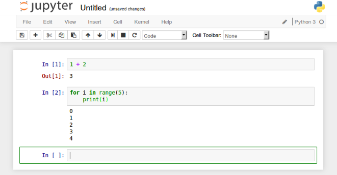
As previously, the code is evaluated and the results are dislayed properly. You may notice there is no Out[2] this time. This is because we printed the results, and no value was returned.
One very interesting feature of the notebook is that you can go back in a cell, change it and reevaluate it again, thus updating your whole document. Try this by going back to the first cell, changing 1 + 2 to 2 + 3, and reevaulating the cell, by pressing Shift + Enter. You will notice the result was updated to 5 as soon as you evaluated the cell. This can be very powerful when you want to explore data or test an equation with different parameters without having to reevaluate your whole script. You can, however, reevaluate the whole notebook at once, by going to Cell -> Run all.
Now that we’ve seen how to enter code, why not try and get a more beautiful and explanatory notebook? To do this, we will use other types of cells, the Header and Markdown cells.
First, let’s add a title to our notebook at the very top. To do that, select the first cell, then click Insert -> Insert cell above. As you can see, a new cell was added at the very top of your document. However, this looks exactly like the previous one. Let’s make it a title cell by clicking on the cell type menu, in the shortcut toolbar:
![]()
You then change it to Heading. A pop-up will be displayed explaining how to create different levels of titles, and you will be left with a different type of cell:

This cell starts with a # sign, meaning this is a level one title. If you want to make subtitles, you can just use the following notation (explained in the pop-up showing up when changing the cell type):
# : First level title
## : Second level title
### : Third level title
...
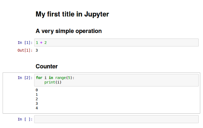
Write your title after the #, then evaluate the cell. You will see the display changing to show a very nice looking title. I added a few other title cells as an example, and an exercise for you:
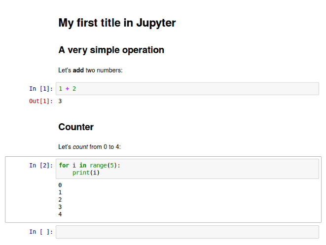
After adding our titles, let’s add a few explanations about what we do in each code cell. For this, we will add a cell where we want it to be, and then change its type to Markdown. Then, evaluate your cell. That’s it: your text is displayed beautifully!
To finish this first introduction, you can rename your notebook by going to File -> Rename and inputing the new name of your notebook. It will then be displayed on the top left of your window, next to the Jupyter logo.
In the next part of this introduction, we will go deeper in the capabilities of the notebook and the integration with other Python libraries.
Click here to carry on reading now!
About the author
Marin Gilles is a PhD student in Physics, in Dijon, France. A large part of his work is dedicated to physical simulations for which he developed his own simulation framework using Python, and contributed to open-source libraries such as Matplotlib or IPython.


