Face recognition using siamese networks [Tutorial]
Read more
Face recognition using siamese networks [Tutorial]
Prasad Ramesh
660 min read
2019-02-25 02:00:16
0 Likes
0 Comments
A siamese network is a special type of neural network and it is one of the simplest and most popularly used one-shot learning algorithms. One-shot learning is a technique where we learn from only one training example per class. So, a siamese network is predominantly used in applications where we don't have many data points in each class. For instance, let's say we want to build a face recognition model for our organization and about 500 people are working in our organization.
If we want to build our face recognition model using a Convolutional Neural Network (CNN) from scratch, then we need many images of all of these 500 people for training the network and attaining good accuracy. But apparently, we will not have many images for all of these 500 people and so it is not feasible to build a model using a CNN or any deep learning algorithm unless we have sufficient data points. So, in these kinds of scenarios, we can resort to a sophisticated one-shot learning algorithm such as a siamese network, which can learn from fewer data points.
Siamese networks basically consist of two symmetrical neural networks both sharing the same weights and architecture and both joined together at the end using some energy function, E. The objective of our siamese network is to learn whether two input values are similar or dissimilar.
We will understand the siamese network by building a face recognition model. The objective of our network is to understand whether two faces are similar or dissimilar. We use the AT&T Database of Faces, which can be downloaded from the Cambridge University Computer Laboratory website.
This article is an excerpt from a book written by Sudharsan Ravichandiran titled Hands-On Meta-Learningwith Python. In this book, you will learn how to build relation networks and matching networks from scratch.
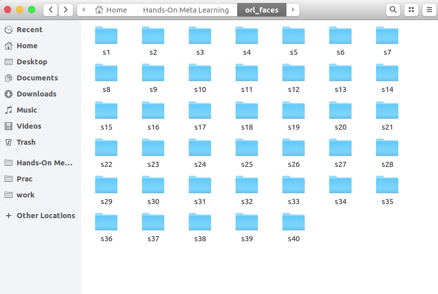
Once you have downloaded and extracted the archive, you can see the folders s1, s2, up to s40, as shown here:
Each of these folders has 10 different images of a single person taken from various angles. For instance, let's open folder s1. As you can see, there are 10 different images of a single person:
We open and check folder s13:
Siamese networks require input values as a pair along with the label, so we have to create our data in such a way. So, we will take two images randomly from the same folder and mark them as a genuine pair and we will take single images from two different folders and mark them as an imposite pair. A sample is shown in the following screenshot; as you can see, a genuine pair has images of the same person and the imposite pair has images of different people:
Once we have our data as pairs along with their labels, we train our siamese network. From the image pair, we feed one image to network A and another image to network B. The role of these two networks is only to extract the feature vectors. So, we use two convolution layers with rectified linear unit (ReLU) activations for extracting the features. Once we have learned the features, we feed the resultant feature vector from both of the networks to the energy function, which measures the similarity; we use Euclidean distance as our energy function. So, we train our network by feeding the image pair to learn the semantic similarity between them. Now, we will see this step by step.
For better understanding, you can check the complete code, which is available as a Jupyter Notebook with an explanation from GitHub.
First, we will import the required libraries:
import re
import numpy as np
from PIL import Image
from sklearn.model_selection import train_test_split
from keras import backend as K
from keras.layers import Activation
from keras.layers import Input, Lambda, Dense, Dropout, Convolution2D, MaxPooling2D, Flatten
from keras.models import Sequential, Model
from keras.optimizers import RMSprop
Now, we define a function for reading our input image. The read_image function takes as input an image and returns a NumPy array:
def read_image(filename, byteorder='>'):
#first we read the image, as a raw file to the buffer
with open(filename, 'rb') as f:
buffer = f.read()
#using regex, we extract the header, width, height and maxval of the image
header, width, height, maxval = re.search(
b"(^P5\s(?:\s*#.*[\r\n])*"
b"(\d+)\s(?:\s*#.*[\r\n])*"
b"(\d+)\s(?:\s*#.*[\r\n])*"
b"(\d+)\s(?:\s*#.*[\r\n]\s)*)", buffer).groups()
#then we convert the image to numpy array using np.frombuffer which interprets buffer as one dimensional array
return np.frombuffer(buffer,
dtype='u1' if int(maxval) < 256 else byteorder+'u2',
count=int(width)*int(height),
offset=len(header)
).reshape((int(height), int(width)))
For an example, let's open one image:
Image.open("data/orl_faces/s1/1.pgm")
When we feed this image to our read_image function, it will return as a NumPy array:
Now, we define another function, get_data, for generating our data. As we know, for the siamese network, data should be in the form of pairs (genuine and imposite) with a binary label.
First, we read the (img1, img2) images from the same directory and store them in the x_genuine_pair array and assign y_genuine to 1. Next, we read the (img1, img2) images from the different directory and store them in the x_imposite pair and assign y_imposite to 0.
Finally, we concatenate both x_genuine_pair and x_imposite to X and y_genuine and y_imposite to Y:
size = 2
total_sample_size = 10000
def get_data(size, total_sample_size):
#read the image
image = read_image('data/orl_faces/s' + str(1) + '/' + str(1) + '.pgm', 'rw+')
#reduce the size
image = image[::size, ::size]
#get the new size
dim1 = image.shape[0]
dim2 = image.shape[1]
count = 0
#initialize the numpy array with the shape of [total_sample, no_of_pairs, dim1, dim2]
x_geuine_pair = np.zeros([total_sample_size, 2, 1, dim1, dim2]) # 2 is for pairs
y_genuine = np.zeros([total_sample_size, 1])
for i in range(40):
for j in range(int(total_sample_size/40)):
ind1 = 0
ind2 = 0
#read images from same directory (genuine pair)
while ind1 == ind2:
ind1 = np.random.randint(10)
ind2 = np.random.randint(10)
# read the two images
img1 = read_image('data/orl_faces/s' + str(i+1) + '/' + str(ind1 + 1) + '.pgm', 'rw+')
img2 = read_image('data/orl_faces/s' + str(i+1) + '/' + str(ind2 + 1) + '.pgm', 'rw+')
#reduce the size
img1 = img1[::size, ::size]
img2 = img2[::size, ::size]
#store the images to the initialized numpy array
x_geuine_pair[count, 0, 0, :, :] = img1
x_geuine_pair[count, 1, 0, :, :] = img2
#as we are drawing images from the same directory we assign label as 1. (genuine pair)
y_genuine[count] = 1
count += 1
count = 0
x_imposite_pair = np.zeros([total_sample_size, 2, 1, dim1, dim2])
y_imposite = np.zeros([total_sample_size, 1])
for i in range(int(total_sample_size/10)):
for j in range(10):
#read images from different directory (imposite pair)
while True:
ind1 = np.random.randint(40)
ind2 = np.random.randint(40)
if ind1 != ind2:
break
img1 = read_image('data/orl_faces/s' + str(ind1+1) + '/' + str(j + 1) + '.pgm', 'rw+')
img2 = read_image('data/orl_faces/s' + str(ind2+1) + '/' + str(j + 1) + '.pgm', 'rw+')
img1 = img1[::size, ::size]
img2 = img2[::size, ::size]
x_imposite_pair[count, 0, 0, :, :] = img1
x_imposite_pair[count, 1, 0, :, :] = img2
#as we are drawing images from the different directory we assign label as 0. (imposite pair)
y_imposite[count] = 0
count += 1
#now, concatenate, genuine pairs and imposite pair to get the whole data
X = np.concatenate([x_geuine_pair, x_imposite_pair], axis=0)/255
Y = np.concatenate([y_genuine, y_imposite], axis=0)
return X, Y
Now, we generate our data and check our data size. As you can see, we have 20,000 data points and, out of these, 10,000 are genuine pairs and 10,000 are imposite pairs:
Next, we split our data for training and testing with 75% training and 25% testing proportions:
Unlock access to the largest independent learning library in Tech for FREE!
Get unlimited access to 7500+ expert-authored eBooks and video courses covering every tech area you can think of.
Renews at $19.99/month. Cancel anytime
x_train, x_test, y_train, y_test = train_test_split(X, Y, test_size=.25)
Now that we have successfully generated our data, we build our siamese network. First, we define the base network, which is basically a convolutional network used for feature extraction. We build two convolutional layers with ReLU activations and max pooling followed by a flat layer:
feat_vecs_a and feat_vecs_b are the feature vectors of our image pair. Next, we feed these feature vectors to the energy function to compute the distance between them, and we use Euclidean distance as our energy function:
In this tutorial, we have learned to build face recognition models using siamese networks. The architecture of siamese networks, basically consists of two identical neural networks both having the same weights and architecture and the output of these networks is plugged into some energy function to understand the similarity. To learn more about meta-learning with Python, check out the book Hands-On Meta-Learning with Python.

 United States
 Great Britain
 India
India
 Germany
 France
 Canada
 Russia
 Spain
Spain
 Brazil
 Australia
 Singapore
 Canary Islands
 Hungary
 Ukraine
 Luxembourg
 Estonia
 Lithuania
 South Korea
 Turkey
 Switzerland
 Colombia
 Taiwan
 Chile
Chile
 Norway
 Ecuador
 Indonesia
 New Zealand
 Cyprus
 Denmark
 Finland
 Poland
 Malta
Malta
 Czechia
 Austria
 Sweden
 Italy
Italy
 Egypt
Egypt
 Belgium
 Portugal
 Slovenia
 Ireland
 Romania
 Greece
 Argentina
 Netherlands
 Bulgaria
 Latvia
 South Africa
 Malaysia
 Japan
Japan
 Slovakia
 Philippines
 Mexico
 Thailand