Cross-Validation strategies for Time Series forecasting [Tutorial]

Time series modeling and forecasting are tricky and challenging. The i.i.d (identically distributed independence) assumption does not hold well to time series data. There is an implicit dependence on previous observations and at the same time, a data leakage from response variables to lag variables is more likely to occur in addition to inherent non-stationarity in the data space. By non-stationarity, we mean flickering changes of observed statistics such as mean and variance. It even gets trickier when taking inherent nonlinearity into consideration. Cross-validation is a well-established methodology for choosing the best model by tuning hyper-parameters or performing feature selection. There are a plethora of strategies for implementing optimal cross-validation. K-fold cross-validation is a time-proven example of such techniques. However, it is not robust in handling time series forecasting issues due to the nature of the data as explained above.

In this tutorial, we shall explore two more techniques for performing cross-validation; time series split cross-validation and blocked cross-validation, which is carefully adapted to solve issues encountered in time series forecasting. We shall use Python 3.5, SciKit Learn, Matplotlib, Numpy, and Pandas. By the end of this tutorial you will have explored the following topics:

• Time Series Split Cross-Validation
• Blocked Cross-Validation
• Grid Search Cross-Validation
• Loss Function
• Elastic Net Regression

Cross-Validation

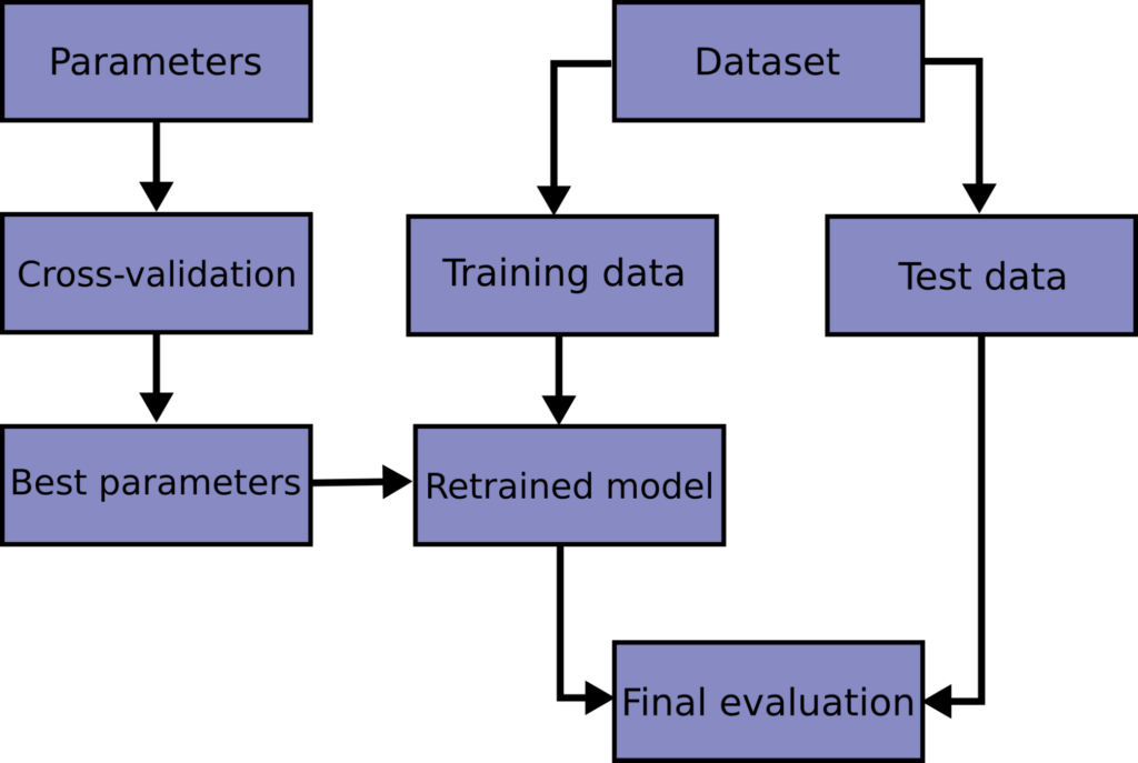
Image Source: scikit-learn.org

First, the data set is split into a training and testing set. The testing set is preserved for evaluating the best model optimized by cross-validation. In k-fold cross-validation, the training set is further split into k folds aka partitions. During each iteration of the cross-validation, one fold is held as a validation set and the remaining k – 1 folds are used for training. This allows us to make the best use of the data available without annihilation. It also allows us to avoid biasing the model towards patterns that may be overly represented in a given fold. Then the error obtained on all folds is averaged and the standard deviation is calculated.

One usually performs cross-validation to find out which settings give the minimum error before training a final model using these elected settings on the complete training set. Flavors of k-fold cross-validations exist, for example, leave-one-out and nested cross-validation. However, these may be the topic of another tutorial.

Grid Search Cross-Validation

One idea to fine-tune the hyper-parameters is to randomly guess the values for model parameters and apply cross-validation to see if they work. This is infeasible as there may be exponential combinations of such parameters. This approach is also called Random Search in the literature.

Grid search works by exhaustively searching the possible combinations of the model’s parameters, but it makes use of the loss function to guide the selection of the values to be tried at each iteration. That is solving a minimization optimization problem. However, in SciKit Learn it explicitly tries all the possible combination which makes it computationally expensive.

When cross-validation is used in the inner loop of the grid search, it is called grid search cross-validation. Hence, the optimization objective becomes minimizing the average loss obtained on the k folds.

R² Loss Function

Choosing the loss function has a very high impact on model performance and convergence. In this tutorial, I would like to introduce to you a loss function, most commonly used in regression tasks. R² loss works by calculating correlation coefficients between the ground truth target values and the response output from the model. The formula is, however, slightly modified so that the range of the function is in the open interval [+1, -∞]. Hence, +1 indicates maximum positive correlation and negative values indicate the opposite. Thus, all the errors obtained in this tutorial should be interpreted as desirable if their value is close to +1. It is worth mentioning that we could have chosen a different loss function such as L1-norm or L2-norm. I would encourage you to try the ideas discussed in this tutorial using other loss functions and observe the difference.

Elastic Net Regression

This also goes in the literature by the name elastic net regularization. Regularization is a very robust technique to avoid overfitting by penalizing large weights or in other words it alters the objective function by emphasizing the errors caused by memorizing the training set. Vanilla linear regression can be tricked into learning the parameters that perform very well on the training set, but yet fail to generalize for unseen new samples.

Both L1-regularization and L2-regularization were incorporated to resolve overfitting and are known in the literature as Lasso and Ridge regression respectively. Due to the critique of both Lasso and Ridge regression, Elastic Net regression was introduced to mix the two models. As a result, some variables’ coefficients are set to zero as per L1-norm and some others are penalized or shrank as per the L2-norm.

This model combines the best from both worlds and the result is a stable, robust, and a sparse model. As a consequence, there are more parameters to be fine-tuned. That’s why this is a good example to demonstrate the power of cross-validation.

Crypto Data Set

I have obtained ETHereum/USD exchange prices for the year 2019 from cryptodatadownload.com which you can get for free from the website or by running the following command:

$ wget http://www.cryptodatadownload.com/cdd/Gemini_ETHUSD_d.csv

Now that you have the CSV file you can import it to Python using Pandas. The daily close price is used as both regressor and response variables. In this setup, I have used a lag of 64 days for regressors and a target of 8 days for responses. That is, given the past 64 days closing prices forecast the next 8 days. Then the resulting nan rows at the tail are dropped as a way to handle missing values.

df = pd.read_csv('./Gemini_ETHUSD_d.csv', skiprows=1)
for i in range(1, STEPS):
    col_name = 'd{}'.format(i)
    df[col_name] = df['d0'].shift(periods=-1 * i)
df = df.dropna()

Next, we split the data frame into two one for the regressors and the other for the responses. And then split both into two one for training and the other for testing.

X = df.iloc[:, :TRAIN_STEPS]
y = df.iloc[:, TRAIN_STEPS:]

X_train = X.iloc[:SPLIT_IDX, :]
y_train = y.iloc[:SPLIT_IDX, :]

X_test = X.iloc[SPLIT_IDX:, :]
y_test = y.iloc[SPLIT_IDX:, :]

Model Design

Let’s define a method that creates an elastic net model from sci-kit learn and since we are going to forecast more than one future time step, let’s use a multi-output regressor wrapper that trains a separate model for each target time step. However, this introduces more demand for computation resources.

def build_model(_alpha, _l1_ratio):
    estimator = ElasticNet(
        alpha=_alpha,
        l1_ratio=_l1_ratio,
        fit_intercept=True,
        normalize=False,
        precompute=False,
        max_iter=16,
        copy_X=True,
        tol=0.1,
        warm_start=False,
        positive=False,
        random_state=None,
        selection='random'
    )

    return MultiOutputRegressor(estimator, n_jobs=4)

Blocked and Time Series Splits Cross-Validation

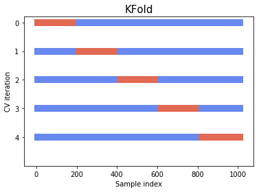
The best way to grasp the intuition behind blocked and time series splits is by visualizing them. The three split methods are depicted in the above diagram. The horizontal axis is the training set size while the vertical axis represents the cross-validation iterations. The folds used for training are depicted in blue and the folds used for validation are depicted in orange. You can intuitively interpret the horizontal axis as time progression line since we haven’t shuffled the dataset and maintained the chronological order.

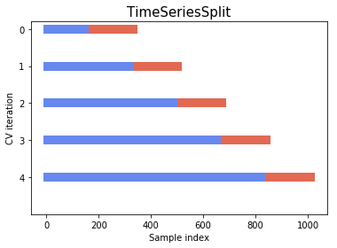
The idea for time series splits is to divide the training set into two folds at each iteration on condition that the validation set is always ahead of the training split. At the first iteration, one trains the candidate model on the closing prices from January to March and validates on April’s data, and for the next iteration, train on data from January to April, and validate on May’s data, and so on to the end of the training set. This way dependence is respected.

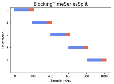
However, this may introduce leakage from future data to the model. The model will observe future patterns to forecast and try to memorize them. That’s why blocked cross-validation was introduced.  It works by adding margins at two positions. The first is between the training and validation folds in order to prevent the model from observing lag values which are used twice, once as a regressor and another as a response. The second is between the folds used at each iteration in order to prevent the model from memorizing patterns from an iteration to the next.

Implementing k-fold cross-validation using sci-kit learn is pretty straightforward, but in the following lines of code, we pass the k-fold splitter explicitly as we will develop the idea further in order to implement other kinds of cross-validation.

model = build_model(_alpha=1.0, _l1_ratio=0.3)
kfcv = KFold(n_splits=5)
scores = cross_val_score(model, X_train, y_train, cv=kfcv, scoring=r2)
print("Loss: {0:.3f} (+/- {1:.3f})".format(scores.mean(), scores.std()))

This outputs:

Loss: -103.076 (+/- 205.979)

The same applies to time series splitter as follows:

model = build_model(_alpha=1.0, _l1_ratio=0.3)
tscv = TimeSeriesSplit(n_splits=5)
scores = cross_val_score(model, X_train, y_train, cv=tscv, scoring=r2)
print("Loss: {0:.3f} (+/- {1:.3f})".format(scores.mean(), scores.std()))

This outputs:

Loss: -9.799 (+/- 19.292)

Sci-kit learn gives us the luxury to define any new types of splitters as long as we abide by its splitter API and inherit from the base splitter.

class BlockingTimeSeriesSplit():
    def __init__(self, n_splits):
        self.n_splits = n_splits
    
    def get_n_splits(self, X, y, groups):
        return self.n_splits
    
    def split(self, X, y=None, groups=None):
        n_samples = len(X)
        k_fold_size = n_samples // self.n_splits
        indices = np.arange(n_samples)

        margin = 0
        for i in range(self.n_splits):
            start = i * k_fold_size
            stop = start + k_fold_size
            mid = int(0.8 * (stop - start)) + start
            yield indices[start: mid], indices[mid + margin: stop]

Then we can use it exactly the same way like before.

model = build_model(_alpha=1.0, _l1_ratio=0.3)
btscv = BlockingTimeSeriesSplit(n_splits=5)
scores = cross_val_score(model, X_train, y_train, cv=btscv, scoring=r2)
print("Loss: {0:.3f} (+/- {1:.3f})".format(scores.mean(), scores.std()))

This outputs:

Loss: -15.527 (+/- 27.488)

Please notice how the loss is different among the different types of splitters. In order to interpret the results correctly, let’s put it to test by using grid search cross-validation to find the optimal values for both regularization parameter alpha and -ratio that controls how much -norm contributes to the regularization. It follows that -norm contributes 1 – .

params = {
    'estimator__alpha':(0.1, 0.3, 0.5, 0.7, 0.9),
    'estimator__l1_ratio':(0.1, 0.3, 0.5, 0.7, 0.9)
}

for i in range(100):
    model = build_model(_alpha=1.0, _l1_ratio=0.3)

    finder = GridSearchCV(
        estimator=model,
        param_grid=params,
        scoring=r2,
        fit_params=None,
        n_jobs=None,
        iid=False,
        refit=False,
        cv=kfcv,  # change this to the splitter subject to test
        verbose=1,
        pre_dispatch=8,
        error_score=-999,
        return_train_score=True
    )

    finder.fit(X_train, y_train)

    best_params = finder.best_params_

Experimental Results

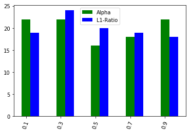
K-Fold Cross-Validation Optimal Parameters

Grid-search cross-validation was run 100 times in order to objectively measure the consistency of the results obtained using each splitter. This way we can evaluate the effectiveness and robustness of the cross-validation method on time series forecasting. As for the k-fold cross-validation, the parameters suggested were almost uniform. That is, it did not really help us in discriminating the optimal parameters since all were equally good or bad.

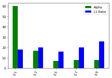
Time Series Split Cross-Validation Optimal Parameters

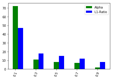
Blocked Cross-Validation Optimal Parameters

However, in both the cases of time series split cross-validation and blocked cross-validation, we have obtained a clear indication of the optimal values for both parameters. In case of blocked cross-validation, the results were even more discriminative as the blue bar indicates the dominance of -ratio optimal value of 0.1.

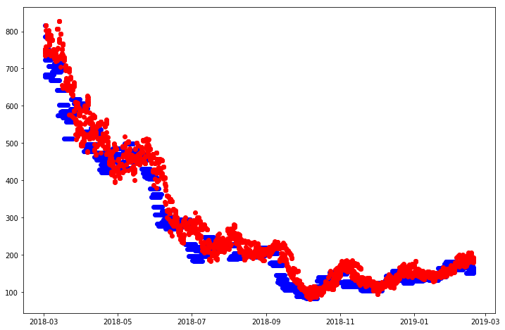
Ground Truth vs Forecasting

After having obtained the optimal values for our model parameters, we can train the model and evaluate it on the testing set. The results, as depicted in the plot above, indicate smooth capture of the trend and minimum error rate.

# optimal model
model = build_model(_alpha=0.1, _l1_ratio=0.1)
# train model
model.fit(X_train, y_train)
# test score
y_predicted = model.predict(X_test)
score = r2_score(y_test, y_predicted, multioutput='uniform_average')
print("Test Loss: {0:.3f}".format(score))

The output is:

Test Loss: 0.925

Ideas for the Curious

In this tutorial, we have demonstrated the power of using the right cross-validation strategy for time-series forecasting. The beauty of machine learning is endless. Here you’re a few ideas to try out and experiment on your own:

• Try using a different more volatile data set
• Try using different lag and target length instead of 64 and 8 days each.
• Try different regression models
• Try different loss functions
• Try RNN models using Keras
• Try increasing or decreasing the blocked splits margins
• Try a different value for k in cross-validation

References

• Jeff Racine,Consistent cross-validatory model-selection for dependent data: hv-block cross-validation,Journal of Econometrics,Volume 99, Issue 1,2000,Pages 39-61,ISSN 0304-4076.
• Dabbs, Beau & Junker, Brian. (2016). Comparison of Cross-Validation Methods for Stochastic Block Models.
• Marcos Lopez de Prado, 2018, Advances in Financial Machine Learning (1st ed.), Wiley Publishing.
• Doctor, Grado DE et al. “New approaches in time series forecasting: methods, software, and evaluation procedures.” (2013).

Learn More

Seize the chance to learn more about time series forecasting techniques, machine learning, trading strategies, and algorithmic trading on my step by step online video course: Hands-on Machine Learning for Algorithmic Trading Bots with Python on PacktPub.

Author Bio

Mustafa Qamar-ud-Din is a machine learning engineer with over 10 years of experience in the software development industry engaged with startups on solving problems in various domains; e-commerce applications, recommender systems, biometric identity control, and event management.

Read Next

Time series modeling: What is it, Why it matters and How it’s used

Implementing a simple Time Series Data Analysis in R

Training RNNs for Time Series Forecasting