(For more resources related to this topic, see here.)
Interactive graphics and animations
This article showcases MATLAB's capabilities for creating interactive graphics and animations. A static graphic is essentially two dimensional. The ability to rotate the axes and change the view, add annotations in real time, delete data, and zoom in or zoom out adds significantly to the user experience, as the brain is able to process and see more from that interaction. MATLAB supports interactivity with the standard zoom, pan features, a powerful set of camera tools to change the data view, data brushing, and axes linking. The set of functionalities accessible from the figure and camera toolbars are outlined briefly as follows:
The steps of interactive exploration can also be recorded and presented as an animation. This is very useful to demonstrate the evolution of the data in time or space or along any dimension where sequence has meaning. Note that some recipes in this article may require you to run the code from the source code files as a whole unit because they were developed as functions. As functions, they are not independently interpretable using the separate code blocks corresponding to each step.
Callback functions
A mouse drag movement from the top-left corner to bottom-right corner is commonly used for zooming in or selecting a group of objects. You can also program a custom behavior to such an interaction event, by using a callback function. When a specific event occurs (for example, you click on a push button or double-click with your mouse), the corresponding callback function executes. Many event properties of graphics handle objects can be used to define callback functions.
In this recipe, you will write callback functions which are essential to implement a slider element to get input from the user on where to create the slice or an isosurface for 3D exploration. You will also see options available to share data between the calling and callback functions.
Getting started
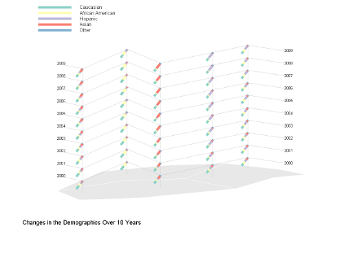
Load the dataset. Split the data into two main sets—userdataA is a structure with variables related to the demographics and userdataB is a structure with variables related to the Income Groups. Now create a nested structure with these two data structures as shown in the following code snippet:
A figure is brought up with a non-standard menu item as highlighted in the following screenshot. Select the By Population item:
Here is the resultant figure:
Continue to explore the other options to fully exercise the interactivity built into this graphic.
How it works...
The function c3165_07_01_callback_functions works as follows:
A custom menu item Data Groups is created, with additional submenu items—By population, By Income Groups, or Show all.
% add main menu item
f = uimenu('Label','Data Groups');
% add sub menu items with additional parameters
uimenu(f,'Label','By Population','Callback','showData',...
'tag','demographics','userdata',userdataAB);
uimenu(f,'Label','By IncomeGroups',...
'Callback','showData','tag','IncomeGroups',...
'userdata',userdataAB);
uimenu(f,'Label','ShowAll','Callback','showData',...
'tag','together','userdata',userdataAB);
You defined the tag name and the callback function for each submenu item above. Having a tag name makes it easier to use the same callback function with multiple objects because you can query the tag name to find out which object initiated the call to the callback function (if you need that information). In this example, the callback function behavior is dependent upon which submenu item was selected. So the tag property allowed you to use the single function showData as callback for all three submenu items and still implement submenu item specific behavior. Alternately, you could also register three different callback functions and use no tag names.
You can specify the value of a callback property in three ways. Here, you gave it a function handle. Alternately, you can supply a string that is a MATLAB command that executes when the callback is invoked. Or, a cell array with the function handle and additional arguments as you will see in the next section.
For passing data between the calling and callback function, you also have three options. Here, you set the userdata property to the variable name that has the data needed by the callback function. Note that the userdata is just one variable and you passed a complicated data structure as userdata to effectively pass multiple values. The user data can be extracted from within the callback function of the object or menu item whose callback is executing as follows:
userdata = get(gcbo,'userdata');
The second alternative to pass data to callback functions is by means of the application data. This does not require you to build a complicated data structure. Depending on how much data you need to pass, this later option may be the faster mechanism. It also has the advantage that the userdata space cannot inadvertently get overwritten by some other function. Use the setappdata function to pass multiple variables. In this recipe, you maintained the main drawing area axis handles and the custom legend axis handles as application data.
This was retrieved each time within the executing callback functions, to clear the graphic as new choices are selected by the user from the custom menu.
mainAxesHandle = getappdata(gcf,'mainAxes');
labelAxesHandles = getappdata(gcf,'labelAxes');
if ~isempty(mainAxesHandle),
cla(mainAxesHandle);
[mainAxesHandle, x, y, ci, cd] = ...
redrawGrid(userdata.years, mainAxesHandle);
else
[mainAxesHandle, x, y, ci, cd] = ...
redrawGrid(userdata.years);
end
if ~isempty(labelAxesHandles)
for ij = 1:length(labelAxesHandles)
cla(labelAxesHandles(ij));
end
end
The third option to pass data to callback functions is at the time of defining the callback property, where you can supply a cell array with the function handle and additional arguments as you will see in the next section. These are local copies of data passed onto the function and will not affect the global values of the variables.
The callback function showData is given below. Functions that you want to use as function handle callbacks must define at least two input arguments in the function definition: the handle of the object generating the callback (the source of the event), the event data structure (can be empty for some callbacks).
function showData(src, evt)
userdata = get(gcbo,'userdata');
if strcmp(get(gcbo,'tag'),'demographics')
% Call grid f drawing code block
% Call showDemographics with relevant inputs
elseif strcmp(get(gcbo,'tag'),'IncomeGroups')
% Call grid drawing code block
% Call showIncomeGroups with relevant inputs
else
% Call grid drawing code block
% Call showDemographics with relevant inputs
% Call showIncomeGroups with relevant inputs
end
function labelAxesHandle = ...
showDemographics(userdata, mainAxesHandle, x, y, cd)
% Function specific code
end
function labelAxesHandle = ...
showIncomeGroups(userdata, mainAxesHandle, x, y, ci)
% Function specific code
end
function [mainAxesHandle x y ci cd] = ...
redrawGrid(years, mainAxesHandle)
% Grid drawing function specific code
end
end
There's more...
This section demonstrates the third option to pass data to callback functions by supplying a cell array with the function handle and additional arguments at the time of defining the callback property. Add a fourth submenu item as follows (uncomment line 45 of the source code):
uimenu(f,'Label',...
'Alternative way to pass data to callback',...
'Callback',{@showData1,userdataAB},'tag','blah');
Define the showData1 function as follows (uncomment lines 49 to 51 of the source code):
function showData1(src, evt, arg1)
disp(arg1.years);
end
Execute the function and see that the value of the years variable are displayed at the MATLAB console when you select the last submenu Alternative way to pass data to callback option.
Takeaways from this recipe:
Use callback functions to define custom responses for each user interaction with your graphic
Use one of the three options for sharing data between calling and callback functions—pass data as arguments with the callback definition, or via the user data space, or via the application data space, as appropriate
See also
Look up MATLAB help on the setappdata, getappdata, userdata property, callback property, and uimenu commands.
Obtaining user input from the graph
User input may be desired for annotating data in terms of adding a label to one or more data points, or allowing user settable boundary definitions on the graphic. This recipe illustrates how to use MATLAB to support these needs.
Getting started
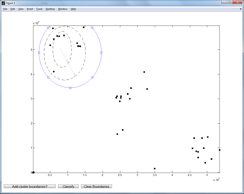
The recipe shows a two-dimensional dataset of intensity values obtained from two different dye fluorescence readings. There are some clearly identifiable clusters of points in this 2D space. The user is allowed to draw boundaries to group points and identify these clusters. Load the data:
load clusterInteractivData
The imellipse function from the MATLAB image processing toolboxTM is used in this recipe. Trial downloads are available from their website.
How to do it...
The function constitutes the following steps:
Set up the user data variables to share the data between the callback functions of the push button elements in this graph:
Define callback for each of the pushbutton elements. The addBound function is for defining the cluster boundaries. The steps are as follows:
% Retrieve the userdata data
userdata = get(gcf,'userdata');
% Allow a maximum of four cluster boundary definitions
if length(userdata.boundDef)>4
msgbox('A maximum of four clusters allowed!');
return;
end
% Allow user to define a bounding curve
h=imellipse(gca);
% The boundary definition is added to a cell array with
% each element of the array storing the boundary def.
userdata.boundDef{length(userdata.boundDef)+1} = ...
h.getPosition;
set(gcf,'userdata',userdata);
The classifyPts function draws points enclosed in a given boundary with a unique symbol per boundary definition. The logic used in this classification function is simple and will run into difficulties with complex boundary definitions. However, that is ignored as that is not the focus of this recipe. Here, first find points whose coordinates lie in the range defined by the coordinates of the boundary definition. Then, assign a unique symbol to all points within that boundary:
Unlock access to the largest independent learning library in Tech for FREE!
Get unlimited access to 7500+ expert-authored eBooks and video courses covering every tech area you can think of.
Renews at $19.99/month. Cancel anytime
for i = 1:length(userdata.boundDef)
pts = ...
find( (userdata.X>(userdata.boundDef{i}(:,1)))& ...
(userdata.X<(userdata.boundDef{i}(:,1)+ ...
userdata.boundDef{i}(:,3))) &...
(userdata.Y>(userdata.boundDef{i}(:,2)))& ...
(userdata.Y<(userdata.boundDef{i}(:,2)+ ...
userdata.boundDef{i}(:,4))));
userdata.Calls(pts) = i;
plot(userdata.X(pts),userdata.Y(pts), ...
[userdata.colorChoice{i} '.'], ...
'Markersize',18); hold on;
end
The clearBounds function clears the drawn boundaries and removes the clustering based upon those boundary definitions.
function clearBounds(src, evt)
cla;
userdata = get(gcf,'userdata');
userdata.boundDef = [];
set(gcf,'userdata',userdata);
plot(userdata.X,userdata.Y,'k.','Markersize',18);
hold on;
end
Run the code and define cluster boundaries using the mouse. Note that until you click the on the Classify button, classification does not occur. Here is a snapshot of how it looks (the arrow and dashed boundary is used to depict the cursor movement from user interaction):
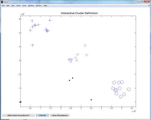
Initiate a classification by clicking on Classify.
The graph will respond by re-drawing all points inside the constructed boundary with a specific symbol:
How it works...
This recipe illustrates how user input is obtained from the graphical display in order to impact the results produced. The image processing toolbox has several such functions that allow user to provide input by mouse clicks on the graphical display—such as imellipse for drawing elliptical boundaries, and imrect for drawing rectangular boundaries. You can refer to the product pages for more information.
Takeaways from this recipe:
Obtain user input directly via the graph in terms of data point level annotations and/or user settable boundary definitions
See also
Look up MATLAB help on the imlineimpoly, imfreehandimrect, and imelli pseginput commands.
Linked axes and data brushing
MATLAB allows creation of programmatic links between the plot and the data sources and linking different plots together. This feature is augmented by support for data brushing, which is a way to select data and mark it up to distinguish from others. Linking plots to their data source allows you to manipulate the values in the variables and have the plot automatically get updated to reflect the changes. Linking between axes enables actions such as zoom or pan to simultaneously affect the view in all linked axes. Data brushing allows you to directly manipulate the data on the plot and have the linked views reflect the effect of that manipulation and/or selection. These features can provide a live and synchronized view of different aspects of your data.
Getting ready
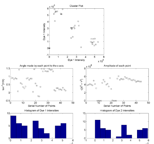
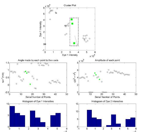
You will use the same cluster data as the previous recipe. Each point is denoted by an x and y value pair. The angle of each point can be computed as the inverse tangent of the ratio of the y value to the x value. The amplitude of each point can be computed as the square root of the sum of squares of the x and y values. The main panel in row 1 show the data in a scatter plot. The two plots in the second row have the angle and amplitude values of each point respectively. The fourth and fifth panels in the third row are histograms of the x and y values respectively. Load the data and calculate the angle and amplitude data as described earlier:
load clusterInteractivData
data(:,1) = X;
data(:,2) = Y;
data(:,3) = atan(Y./X);
data(:,4) = sqrt(X.^2 + Y.^2);
clear X Y
axes('position',[.0682 .3009 .4051 .2240], ...
'Fontsize',12);
scatter(1:length(data),data(:,3),'ks',...
'YDataSource','data(:,3)');
box on;
xlabel('Serial Number of Points');
title('Angle made by each point to the x axis');
ylabel('tan^{-1}(Y/X)');
Plot the amplitude data:
axes('position',[.5588 .3009 .4051 .2240], ...
'Fontsize',12);
scatter(1:length(data),data(:,4),'ks', ...
'YDataSource','data(:,4)');
box on;
xlabel('Serial Number of Points');
title('Amplitude of each point');
ylabel('{surd(X^2 + Y^2)}');
Programmatically, turn brushing on and set the brush color to green:
h = brush;
set(h,'Color',[0 1 0],'Enable','on');
Use mouse movements to brush a set of points. You could do this on any one of the first three panels and observe the impact on corresponding points in the other graphs by its turning green. (The arrow and dashed boundary is used to depict the cursor movement from user interaction in the following figure):
How it works...
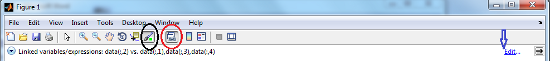
Because brushing is turned on, when you focus the mouse on any of the graph areas, a cross hair shows up at the cursor. You can drag to select an area of the graph. Points falling within the selected area are brushed to the color green, for the graphs on rows 1 and 2. Note that nothing is highlighted on the histograms at this point. This is because the x and y data source for the histograms is not correctly linked to the data source variables yet. For the other graphs, you programmatically set their x and y data source via the XDataSource and the YDataSource properties. You can also define the source data variables to link to a graphic and turn brushing on by using the icons from the figure toolbar as shown in the following screenshot. The first circle highlights the brush button; the second circle highlights the link data button. You can click on the Edit link pointed by the arrow to exactly define the x and y sources:
There's more...
To define the source data variables to link to a graphic and turn brushing on by using the icons from the Figure toolbar, do as follows:
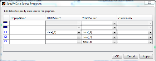
Clicking on Edit (pointed to in preceding figure) will bring up the following window:
Enter data(:,1) in the YDataSource column for row 1 and data(:,2) in the YDataSource column for row 2.
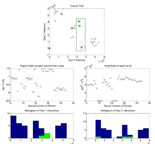
Now try brushing again. Observe that bins of the histogram get highlights in a bottom up order as corresponding points get selected (again, the arrow and dashed boundary is used to depict the cursor movement from user interaction):
Link axes together to simultaneously investigate multiple aspects of the same data point. For example, in this step you plot the cluster data alongside a random quality value for each point of the data. Link the axes such that zoom and pan functions on either will impact the axes of the other linked axes:

 United States
 Great Britain
 India
India
 Germany
 France
 Canada
 Russia
 Spain
Spain
 Brazil
 Australia
 Singapore
 Canary Islands
 Hungary
 Ukraine
 Luxembourg
 Estonia
 Lithuania
 South Korea
 Turkey
 Switzerland
 Colombia
 Taiwan
 Chile
Chile
 Norway
 Ecuador
 Indonesia
 New Zealand
 Cyprus
 Denmark
 Finland
 Poland
 Malta
Malta
 Czechia
 Austria
 Sweden
 Italy
Italy
 Egypt
Egypt
 Belgium
 Portugal
 Slovenia
 Ireland
 Romania
 Greece
 Argentina
 Netherlands
 Bulgaria
 Latvia
 South Africa
 Malaysia
 Japan
Japan
 Slovakia
 Philippines
 Mexico
 Thailand