


A CNN is a combination of two components: a feature extractor module followed by a trainable classifier. The first component includes a stack of convolution, activation, and pooling layers. A dense neural network (DNN) does the classification. Each neuron in a layer is connected to those in the next layer.
This article is an excerpt from the book, Machine Learning Using TensorFlow Cookbook by Alexia Audevart, Konrad Banachewicz and Luca Massaron who are Kaggle Masters and Google Developer Experts.
Implementing a simple CNN
In this section, we will develop a CNN based on the LeNet-5 architecture, which was first introduced in 1998 by Yann LeCun et al. for handwritten and machine-printed character recognition.
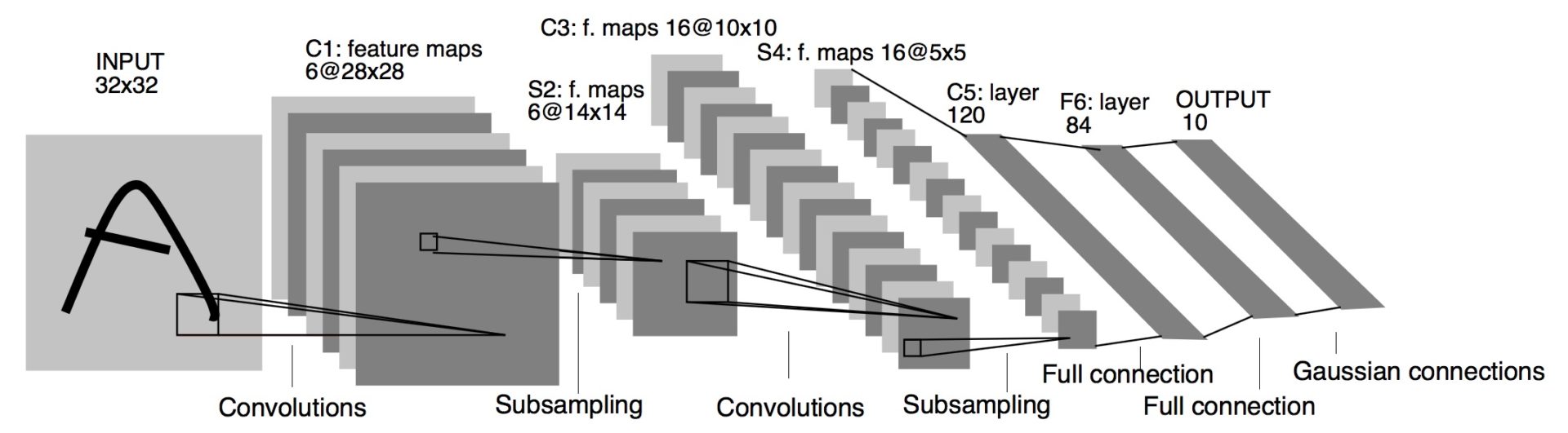
Figure 1: LeNet-5 architecture – Original image published in [LeCun et al., 1998]
This architecture consists of two sets of CNNs composed of convolution-ReLU-max pooling operations used for feature extraction, followed by a flattening layer and two fully connected layers to classify the images. Our goal will be to improve upon our accuracy in predicting MNIST digits.
Getting ready
To access the MNIST data, Keras provides a package (tf.keras.datasets) that has excellent dataset-loading functionalities. (Note that TensorFlow also provides its own collection of ready-to-use datasets with the TF Datasets API.) After loading the data, we will set up our model variables, create the model, train the model in batches, and then visualize loss, accuracy, and some sample digits.
How to do it…
Perform the following steps:
- First, we’ll load the necessary libraries and start a graph session:
import matplotlib.pyplot as plt
import numpy as np
import tensorflow as tf
2. Next, we will load the data and reshape the images in a four-dimensional matrix:
(x_train, y_train), (x_test, y_test) = tf.keras.datasets.mnist.load_data()
# Reshape
x_train = x_train.reshape(-1, 28, 28, 1)
x_test = x_test.reshape(-1, 28, 28, 1)
#Padding the images by 2 pixels
x_train = np.pad(x_train, ((0,0),(2,2),(2,2),(0,0)), 'constant')
x_test = np.pad(x_test, ((0,0),(2,2),(2,2),(0,0)), 'constant')
“Note that the MNIST dataset downloaded here includes training and test datasets. These datasets are composed of the grayscale images (integer arrays with shape (num_sample, 28,28)) and the labels (integers in the range 0-9). We pad the images by 2 pixels since in the LeNet-5 paper input images were 32×32.”
3. Now, we will set the model parameters. Remember that the depth of the image (number of channels) is 1 because these images are grayscale. We’ll also set up a seed to have reproducible results:
image_width = x_train[0].shape[0]
image_height = x_train[0].shape[1]
num_channels = 1 # grayscale = 1 channel
seed = 98
np.random.seed(seed)
tf.random.set_seed(seed)
4. We’ll declare our training data variables and our test data variables. We will have different batch sizes for training and evaluation. You may change these, depending on the physical memory that is available for training and evaluating:
batch_size = 100
evaluation_size = 500
epochs = 300
eval_every = 5
5. We’ll normalize our images to change the values of all pixels to a common scale:
x_train = x_train / 255
x_test = x_test/ 255
6. Now we’ll declare our model. We will have the feature extractor module composed of two convolutional/ReLU/max pooling layers followed by the classifier with fully connected layers. Also, to get the classifier to work, we flatten the output of the feature extractor module so we can use it in the classifier. Note that we use a softmax activation function at the last layer of the classifier. Softmax turns numeric output (logits) into probabilities that sum to one.
input_data = tf.keras.Input(dtype=tf.float32, shape=(image_width,image_height, num_channels), name=“INPUT”)
 # First Conv-ReLU-MaxPool Layer
conv1 = tf.keras.layers.Conv2D(filters=6,
                               kernel_size=5,
                               padding='VALID',
                               activation="relu",
                               name="C1")(input_data)

max_pool1 = tf.keras.layers.MaxPool2D(pool_size=2,
                                      strides=2,
                                      padding='SAME',
                                      name="S1")(conv1)

# Second Conv-ReLU-MaxPool Layer
conv2 = tf.keras.layers.Conv2D(filters=16,
                               kernel_size=5,
                               padding='VALID',
                               strides=1,
                               activation="relu",
                               name="C3")(max_pool1)

max_pool2 = tf.keras.layers.MaxPool2D(pool_size=2,
                                      strides=2,
                                      padding='SAME',
                                      name="S4")(conv2)

# Flatten Layer
flatten = tf.keras.layers.Flatten(name="FLATTEN")(max_pool2)

# First Fully Connected Layer
fully_connected1 = tf.keras.layers.Dense(units=120,
                                         activation="relu",
                                         name="F5")(flatten)

# Second Fully Connected Layer
fully_connected2 = tf.keras.layers.Dense(units=84,
                                         activation="relu",
                                         name="F6")(fully_connected1)

# Final Fully Connected Layer
final_model_output = tf.keras.layers.Dense(units=10,
                                           activation="softmax",
                                           name="OUTPUT"
                                           )(fully_connected2)

model = tf.keras.Model(inputs= input_data, outputs=final_model_output)
7. Next, we will compile the model using an Adam (Adaptive Moment Estimation) optimizer. Adam uses Adaptive Learning Rates and Momentum that allow us to get to local minima faster, and so, to converge faster. As our targets are integers and not in a one-hot encoded format, we will use the sparse categorical cross-entropy loss function. Then we will also add an accuracy metric to determine how accurate the model is on each batch.
model.compile(
    optimizer="adam",
    loss="sparse_categorical_crossentropy",
    metrics=["accuracy"]
8. Next, we print a string summary of our network.
model.summary()
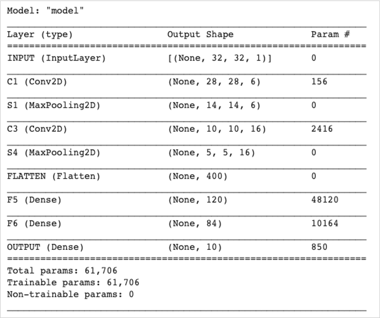
Figure 4: The LeNet-5 architecture
The LeNet-5 model has 7 layers and contains 61,706 trainable parameters. So, let’s go to train the model.
9. We can now start training our model. We loop through the data in randomly chosen batches. Every so often, we choose to evaluate the model on the train and test batches and record the accuracy and loss. We can see that, after 300 epochs, we quickly achieve 96%-97% accuracy on the test data:
train_loss = []
train_acc = []
test_acc = []
for i in range(epochs):
    rand_index = np.random.choice(len(x_train), size=batch_size)
    rand_x = x_train[rand_index]
    rand_y = y_train[rand_index]

    history_train = model.train_on_batch(rand_x, rand_y)

    if (i+1) % eval_every == 0:
        eval_index = np.random.choice(len(x_test), size=evaluation_size)
        eval_x = x_test[eval_index]
        eval_y = y_test[eval_index]

        history_eval = model.evaluate(eval_x,eval_y)

        # Record and print results
        train_loss.append(history_train[0])
        train_acc.append(history_train[1])
        test_acc.append(history_eval[1])
        acc_and_loss = [(i+1), history_train
 [0], history_train[1], history_eval[1]]
        acc_and_loss = [np.round(x,2) for x in acc_and_loss]
        print('Epoch # {}. Train Loss: {:.2f}. Train Acc (Test Acc): {:.2f} ({:.2f})'.format(*acc_and_loss))
10. This results in the following output:
Epoch # 5. Train Loss: 2.19. Train Acc (Test Acc): 0.23 (0.34)
Epoch # 10. Train Loss: 2.01. Train Acc (Test Acc): 0.59 (0.58)
Epoch # 15. Train Loss: 1.71. Train Acc (Test Acc): 0.74 (0.73)
Epoch # 20. Train Loss: 1.32. Train Acc (Test Acc): 0.73 (0.77)
 ...
Epoch # 290. Train Loss: 0.18. Train Acc (Test Acc): 0.95 (0.94)
Epoch # 295. Train Loss: 0.13. Train Acc (Test Acc): 0.96 (0.96)
Epoch # 300. Train Loss: 0.12. Train Acc (Test Acc): 0.95 (0.97)
11. The following is the code to plot the loss and accuracy using Matplotlib:
# Matlotlib code to plot the loss and accuracy
eval_indices = range(0, epochs, eval_every)
# Plot loss over time
plt.plot(eval_indices, train_loss, 'k-')
plt.title('Loss per Epoch')
plt.xlabel('Epoch')
plt.ylabel('Loss')
plt.show()

# Plot train and test accuracy
plt.plot(eval_indices, train_acc, 'k-', label='Train Set Accuracy')
plt.plot(eval_indices, test_acc, 'r--', label='Test Set Accuracy')
plt.title('Train and Test Accuracy')
plt.xlabel('Epoch')
plt.ylabel('Accuracy')
plt.legend(loc='lower right')
plt.show()
We then get the following plots:
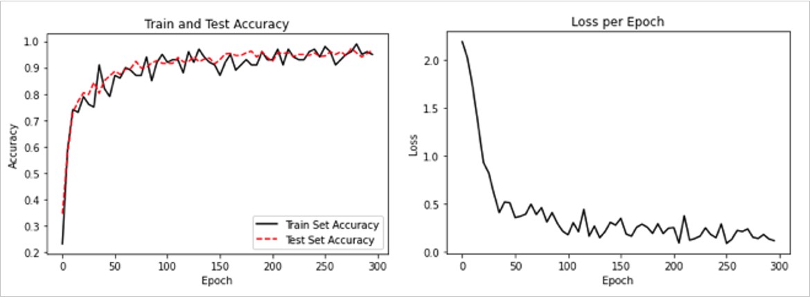
Figure 5: The left plot is the train and test set accuracy across our 300 training epochs. The right plot is the softmax loss value over 300 epochs.
- If we want to plot a sample of the latest batch results, here is the code to plot a sample consisting of six of the latest results:
# Plot some samples and their predictions
actuals = y_test[30:36]
preds = model.predict(x_test[30:36])
predictions = np.argmax(preds,axis=1)
images = np.squeeze(x_test[30:36])

Nrows = 2
Ncols = 3
for i in range(6):
    plt.subplot(Nrows, Ncols, i+1)
    plt.imshow(np.reshape(images[i], [32,32]), cmap='Greys_r')
    plt.title('Actual: ' + str(actuals[i]) + ' Pred: ' + str(predictions[i]),
                               fontsize=10)
    frame = plt.gca()
    frame.axes.get_xaxis().set_visible(False)
    frame.axes.get_yaxis().set_visible(False)

plt.show()
We get the following output for the code above:
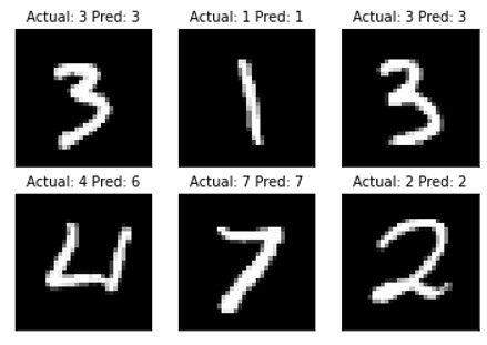
Figure 6: A plot of six random images with the actual and predicted values in the title. The lower-left picture was predicted to be a 6, when in fact it is a 4.
Using a simple CNN, we achieved a good result in accuracy and loss for this dataset.
How it works…
We increased our performance on the MNIST dataset and built a model that quickly achieves about 97% accuracy while training from scratch. Our features extractor module is a combination of convolutions, ReLU, and max pooling. Our classifier is a stack of fully connected layers. We trained in batches of size 100 and looked at the accuracy and loss across the epochs. Finally, we also plotted six random digits and found that the model prediction fails to predict one image. The model predicts a 6 when in fact it’s a 4.
CNN does very well with image recognition. Part of the reason for this is that the convolutional layer creates its low-level features that are activated when they come across a part of the image that is important. This type of model creates features on its own and uses them for prediction.
Summary:
This article highlights how to create a simple CNN, based on the LeNet-5 architecture. The recipes cited in the book Machine Learning Using TensorFlow enable you to perform complex data computations and gain valuable insights into data.
About the Authors
Alexia Audevart, is a Google Developer Expert in machine learning and the founder of Datactik. She is a data scientist and helps her clients solve business problems by making their applications smarter.
Konrad Banachewicz holds a PhD in statistics from Vrije Universiteit Amsterdam. He is a lead data scientist at eBay and a Kaggle Grandmaster.
Luca Massaron is a Google Developer Expert in machine learning with more than a decade of experience in data science. He is also a Kaggle master who reached number 7 for his performance in data science competitions.


