


Budget and demand forecasting are important aspects of any finance team. Budget forecasting is the outcome, and demand forecasting is one of its components.
In this article, we understand the Markov model for forecasting and budgeting in finance.
This article is an excerpt from a book written by Harish Gulati titled SAS for Finance.
Understanding problem of budget and demand forecasting
While a few decades ago, retail banks primarily made profits by leveraging their treasury office, recent years have seen fee income become a major source of profitability. Accepting deposits from customers and lending to other customers is one of the core functions of the treasury. However, charging for current or savings accounts with add-on facilities such as breakdown cover, mobile, and other insurances, and so on, has become a lucrative avenue for banks. One retail bank has a plain vanilla classic bank account, mid-tier premier, and a top-of-the-range, benefits included a platinum account.
The classic account is offered free and the premier and platinum have fees of $10 and $20 per month respectively. The marketing team has just relaunched the fee-based accounts with added benefits. The finance team wanted a projection of how much revenue could be generated via the premier and the platinum accounts.
Solving with Markovian model approach
Even though we have three types of account, the classic, premier, and the platinum, it doesn’t mean that we are only going to have nine transition types possible as in Figure 4.1. There are customers who will upgrade, but also others who may downgrade. There could also be some customers who leave the bank and at the same time there will be a constant inflow of new customers. Let’s evaluate the transition states flow for our business problem:
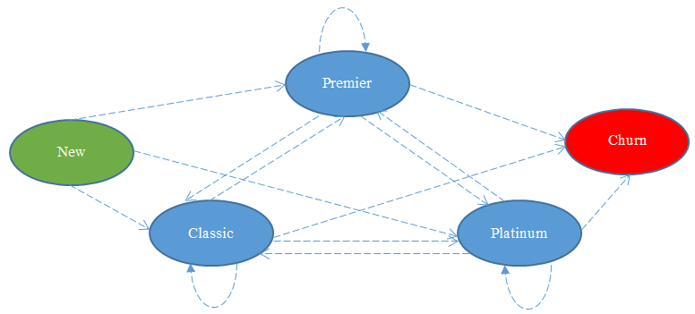
In Figure 4.2, we haven’t jotted down the transition probability between each state. We can try to do this by looking at the historical customer movements, to arrive at the transitional probability. Be aware that most business managers would prefer to use their instincts while assigning transitional probabilities.
They may achieve some merit in this approach, as the managers may be able to incorporate the various factors that may have influenced the customer movements between states. A promotion offering 40% off the platinum account (effective rate $12/month, down from $20/month) may have ensured that more customers in the promotion period opted for the platinum account than the premier offering ($10/month).
Let’s examine the historical data of customer account preferences. The data is compiled for the years 2008 – 2018. This doesn’t account for any new customers joining after January 1, 2008 and also ignores information on churned customers in the period of interest.
Figure 4.3 consists of customers who have been with the bank since 2008:
| Active customer counts (Millions) | ||||
| Year | Classic (Cl) | Premium (Pr) | Platinum (Pl) | Total customers |
| 2008 H1 | 30.68 | 5.73 | 1.51 | 37.92 |
| 2008 H2 | 30.65 | 5.74 | 1.53 | 37.92 |
| 2009 H1 | 30.83 | 5.43 | 1.66 | 37.92 |
| 2009 H2 | 30.9 | 5.3 | 1.72 | 37.92 |
| 2010 H1 | 31.1 | 4.7 | 2.12 | 37.92 |
| 2010 H2 | 31.05 | 4.73 | 2.14 | 37.92 |
| 2011 H1 | 31.01 | 4.81 | 2.1 | 37.92 |
| 2011 H2 | 30.7 | 5.01 | 2.21 | 37.92 |
| 2012 H1 | 30.3 | 5.3 | 2.32 | 37.92 |
| 2012 H2 | 29.3 | 6.4 | 2.22 | 37.92 |
| 2013 H1 | 29.3 | 6.5 | 2.12 | 37.92 |
| 2013 H2 | 28.8 | 7.3 | 1.82 | 37.92 |
| 2014 H1 | 28.8 | 8.1 | 1.02 | 37.92 |
| 2014 H2 | 28.7 | 8.3 | 0.92 | 37.92 |
| 2015 H1 | 28.6 | 8.34 | 0.98 | 37.92 |
| 2015 H2 | 28.4 | 8.37 | 1.15 | 37.92 |
| 2016 H1 | 27.6 | 9.01 | 1.31 | 37.92 |
| 2016 H2 | 26.5 | 9.5 | 1.92 | 37.92 |
| 2017 H1 | 26 | 9.8 | 2.12 | 37.92 |
| 2017 H2 | 25.3 | 10.3 | 2.32 | 37.92 |
Since we are only considering active customers, and no new customers are joining or leaving the bank, we can calculate the number of customers moving from one state to another using the data in Figure 4.3:
| Customer movement count to next year (Millions) | ||||||||||
| Year | Cl-Cl | Cl-Pr | Cl-Pl | Pr-Pr | Pr-Cl | Pr-Pl | Pl-Pl | Pl-Cl | Pl-Pr | Total customers |
| 2008 H1 | – | – | – | – | – | – | – | – | – | – |
| 2008 H2 | 30.28 | 0.2 | 0.2 | 5.5 | 0 | 0.23 | 1.1 | 0.37 | 0.04 | 37.92 |
| 2009 H1 | 30.3 | 0.1 | 0.25 | 5.1 | 0.53 | 0.11 | 1.3 | 0 | 0.23 | 37.92 |
| 2009 H2 | 30.5 | 0.32 | 0.01 | 4.8 | 0.2 | 0.43 | 1.28 | 0.2 | 0.18 | 37.92 |
| 2010 H1 | 30.7 | 0.2 | 0 | 4.3 | 0 | 1 | 1.12 | 0.4 | 0.2 | 37.92 |
| 2010 H2 | 30.7 | 0.2 | 0.2 | 4.11 | 0.35 | 0.24 | 1.7 | 0 | 0.42 | 37.92 |
| 2011 H1 | 30.9 | 0 | 0.15 | 4.6 | 0 | 0.13 | 1.82 | 0.11 | 0.21 | 37.92 |
| 2011 H2 | 30.2 | 0.8 | 0.01 | 3.8 | 0.1 | 0.91 | 1.29 | 0.4 | 0.41 | 37.92 |
| 2012 H1 | 30.29 | 0.4 | 0.01 | 4.9 | 0.01 | 0.1 | 2.21 | 0 | 0 | 37.92 |
| 2012 H2 | 29.3 | 0.9 | 0.1 | 5.3 | 0 | 0 | 2.12 | 0 | 0.2 | 37.92 |
| 2013 H1 | 29.2 | 0.1 | 0 | 6.1 | 0.1 | 0.2 | 1.92 | 0 | 0.3 | 37.92 |
| 2013 H2 | 28.6 | 0.3 | 0.4 | 6.5 | 0 | 0 | 1.42 | 0.2 | 0.5 | 37.92 |
| 2014 H1 | 28.7 | 0.1 | 0 | 7.2 | 0.1 | 0 | 1.02 | 0 | 0.8 | 37.92 |
| 2014 H2 | 28.7 | 0 | 0.1 | 8.1 | 0 | 0 | 0.82 | 0 | 0.2 | 37.92 |
| 2015 H1 | 28.6 | 0 | 0.1 | 8.3 | 0 | 0 | 0.88 | 0 | 0.04 | 37.92 |
| 2015 H2 | 28.3 | 0 | 0.3 | 8 | 0.1 | 0.24 | 0.61 | 0 | 0.37 | 37.92 |
| 2016 H1 | 27.6 | 0.8 | 0 | 8.21 | 0 | 0.16 | 1.15 | 0 | 0 | 37.92 |
| 2016 H2 | 26 | 1 | 0.6 | 8.21 | 0.5 | 0.3 | 1.02 | 0 | 0.29 | 37.92 |
| 2017 H1 | 25 | 0.5 | 1 | 8 | 0.5 | 1 | 0.12 | 0.5 | 1.3 | 37.92 |
| 2017 H2 | 25.3 | 0.1 | 0.6 | 9 | 0 | 0.8 | 0.92 | 0 | 1.2 | 37.92 |
In Figure 4.4, we can see the customer movements between various states. We don’t have the movements for the first half of 2008 as this is the start of the series. In the second half of 2008, we see that 30.28 out of 30.68 million customers (30.68 is the figure from the first half of 2008) were still using a classic account.
However, 0.4 million customers moved away to premium and platinum accounts. The total customers remain constant at 37.92 million as we have ignored new customers joining and any customers who have left the bank. From this table, we can calculate the transition probabilities for each state:
| Year | Cl-Cl | Cl-Pr | Cl-Pl | Pr-Pr | Pr-Cl | Pr-Pl | Pl-Pl | Pl-Cl | Pl-Pr |
| 2008 H2 | 98.7% | 0.7% | 0.7% | 96.0% | 0.0% | 4.0% | 72.8% | 24.5% | 2.6% |
| 2009 H1 | 98.9% | 0.3% | 0.8% | 88.9% | 9.2% | 1.9% | 85.0% | 0.0% | 15.0% |
| 2009 H2 | 98.9% | 1.0% | 0.0% | 88.4% | 3.7% | 7.9% | 77.1% | 12.0% | 10.8% |
| 2010 H1 | 99.4% | 0.6% | 0.0% | 81.1% | 0.0% | 18.9% | 65.1% | 23.3% | 11.6% |
| 2010 H2 | 98.7% | 0.6% | 0.6% | 87.4% | 7.4% | 5.1% | 80.2% | 0.0% | 19.8% |
| 2011 H1 | 99.5% | 0.0% | 0.5% | 97.3% | 0.0% | 2.7% | 85.0% | 5.1% | 9.8% |
| 2011 H2 | 97.4% | 2.6% | 0.0% | 79.0% | 2.1% | 18.9% | 61.4% | 19.0% | 19.5% |
| 2012 H1 | 98.7% | 1.3% | 0.0% | 97.8% | 0.2% | 2.0% | 100.0% | 0.0% | 0.0% |
| 2012 H2 | 96.7% | 3.0% | 0.3% | 100.0% | 0.0% | 0.0% | 91.4% | 0.0% | 8.6% |
| 2013 H1 | 99.7% | 0.3% | 0.0% | 95.3% | 1.6% | 3.1% | 86.5% | 0.0% | 13.5% |
| 2013 H2 | 97.6% | 1.0% | 1.4% | 100.0% | 0.0% | 0.0% | 67.0% | 9.4% | 23.6% |
| 2014 H1 | 99.7% | 0.3% | 0.0% | 98.6% | 1.4% | 0.0% | 56.0% | 0.0% | 44.0% |
| 2014 H2 | 99.7% | 0.0% | 0.3% | 100.0% | 0.0% | 0.0% | 80.4% | 0.0% | 19.6% |
| 2015 H1 | 99.7% | 0.0% | 0.3% | 100.0% | 0.0% | 0.0% | 95.7% | 0.0% | 4.3% |
| 2015 H2 | 99.0% | 0.0% | 1.0% | 95.9% | 1.2% | 2.9% | 62.2% | 0.0% | 37.8% |
| 2016 H1 | 97.2% | 2.8% | 0.0% | 98.1% | 0.0% | 1.9% | 100.0% | 0.0% | 0.0% |
| 2016 H2 | 94.2% | 3.6% | 2.2% | 91.1% | 5.5% | 3.3% | 77.9% | 0.0% | 22.1% |
| 2017 H1 | 94.3% | 1.9% | 3.8% | 84.2% | 5.3% | 10.5% | 6.2% | 26.0% | 67.7% |
| 2017 H2 | 97.3% | 0.4% | 2.3% | 91.8% | 0.0% | 8.2% | 43.4% | 0.0% | 56.6% |
In Figure 4.5, we have converted the transition counts into probabilities. If 30.28 million customers in 2008 H2 out of 30.68 million customers in 2008 H1 are retained as classic customers, we can say that the retention rate is 98.7%, or the probability of customers staying with the same account type in this instance is .987.
Using these details, we can compute the average transition between states across the time series. These averages can be used as the transition probabilities that will be used in the transition matrix for the model:
| Cl | Pr | Pl | |
| Cl | 98.2% | 1.1% | 0.8% |
| Pr | 2.0% | 93.2% | 4.8% |
| Pl | 6.3% | 20.4% | 73.3% |
The probability of classic customers retaining the same account type between semiannual time periods is 98.2%. The lowest retain probability is for platinum customers as they are expected to transition to another customer account type 26.7% of the time. Let’s use the transition matrix in Figure 4.6 to run our Markov model.
Use this code for Data setup:
DATA Current;
input date CL PR PL;
datalines;
2017.2 25.3 10.3 2.32
;
Run;

Data Netflow;
input date CL PR PL;
datalines;
2018.1 0.21 0.1 0.05
2018.2 0.22 0.16 0.06
2019.1 .24 0.18 0.08
2019.2 0.28 0.21 0.1
2020.1 0.31 0.23 0.14
;
Run;

Data TransitionMatrix;
input CL PR PL;
datalines;
0.98 0.01 0.01
0.02 0.93 0.05
0.06 0.21 0.73
;
Run;
In the current data set, we have chosen the last available data point, 2017 H2. This is the base position of customer counts across classic, premium, and platinum accounts. While calculating the transition matrix, we haven’t taken into account new joiners or leavers. However, to enable forecasting we have taken 2017 H2 as our base position. The transition matrix seen in Figure 4.6 has been input as a separate dataset.
Markov model code
PROC IML;
use Current; read all into Current;
use Netflow; read all into Netflow;
use TransitionMatrix; read all into TransitionMatrix;


Current = Current [1,2:4];
Netflow = Netflow [,2:4];

Model_2018_1 = Current * TransitionMatrix + Netflow [1,];
Model_2018_2 = Model_2018_1 * TransitionMatrix + Netflow [1,];
Model_2019_1 = Model_2018_2 * TransitionMatrix + Netflow [1,];
Model_2019_2 = Model_2019_1 * TransitionMatrix + Netflow [1,];
Model_2020_1 = Model_2019_2 * TransitionMatrix + Netflow [1,];

Budgetinputs = Model_2018_1//Model_2018_2//Model_2019_1//Model_2019_2//Model_2020_1;

Create Budgetinputs from Budgetinputs;
append from Budgetinputs;
Quit;

Data Output;
Set Budgetinputs (rename=(Col1=Cl Col2=Pr Col3=Pl));
Run;

Proc print data=output;
Run;
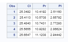
The Markov model has been run and we are able to generate forecasts for all account types for the requested five periods. We can immediately see that there is an increase forecasted for all the account types. This is being driven by the net flow of customers. We have derived the forecasts by essentially using the following equation:
Forecast = Current Period * Transition Matrix + Net Flow
Once the 2018 H1 forecast is derived, we replace the Current Period with the 2018 H1 forecasted number while trying to forecast the 2018 H2 numbers. We are doing this as, based on the 2018 H1 customer counts, the transition probabilities will determine how many customers move across states. This will help generate the forecasted customer count for the required period.
Understanding transition probability
Now, since we have our forecasts let’s take a step back and revisit our business goals. The finance team wants to estimate the revenues from the revamped premium and platinum customer accounts for the next few forecasting periods. As we have seen, one of the important drivers of the forecasting process is the transition probability. This transition probability is driven by historical customer movements, as shown in Figure 4.4.
What if the marketing team doesn’t agree with the transitional probabilities calculated in Figure 4.6? As we discussed, 26.7% of platinum customers aren’t retained in this account type. Since we are not considering customer churn out of the bank, this means that a large proportion of platinum customers downgrade their accounts. One of the reasons the marketing teams revamped the accounts is due to this reason.
The marketing team feels that it will be able to raise the retention rates for platinum customers and want the finance team to run an alternate forecasting scenario. This is, in fact, one of the pros of the Markov model approach as by tweaking the transition probabilities we can run various business scenarios. Let’s compare the base and the alternate scenario forecasts generated in Figure 4.8:
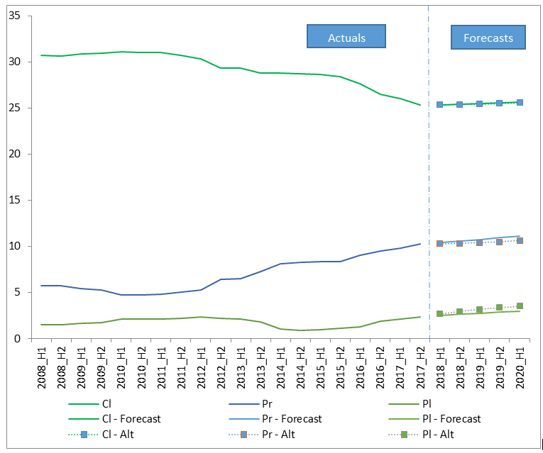
A change in the transition probabilities of how platinum customers moved to various states has brought about a significant change in the forecast for premium and platinum customer accounts. For classic customers, the change in the forecast between the base and the alternate scenario is negligible, as shown in the table in Figure 4.8. The finance team can decide which scenario is best suited for budget forecasting:
| Cl | Pr | Pl | |
| Cl | 98.2% | 1.1% | 0.8% |
| Pr | 2.0% | 93.2% | 4.8% |
| Pl | 5.0% | 15.0% | 80.0% |
To summarize, we learned the Markov model methodology and learned Markov models for forecasting and imputation.
To know more about how to use the other two methodologies such as ARIMA and MCMC for generating forecasts for various business problems, you can check out the book SAS for Finance.


How you calculate Netflow for 2018 onward
Can u explain ?