


Sometimes, R code just isn’t fast enough. Maybe you’ve used profiling to figure out where your bottlenecks are, and you’ve done everything you can think of within R, but your code still isn’t fast enough. In those cases, a useful alternative can be to delegate some parts of the implementation to Fortran or C++. This is an advanced technique that can often prove to be quite useful if know how to program in such languages. In today’s tutorial, we will try to explore techniques to boost R codes and calculations using efficient languages like Fortran and C++.
Delegating code to other languages can address bottlenecks such as the following:
- Loops that can’t be easily vectorized due to iteration dependencies
- Processes that involve calling functions millions of times
- Inefficient but necessary data structures that are slow in R
Delegating code to other languages can provide great performance benefits, but it also incurs the cost of being more explicit and careful with the types of objects that are being moved around. In R, you can get away with simple things such as being imprecise about a number being an integer or a real. In these other languages, you can’t; every object must have a precise type, and it remains fixed for the entire execution.
Boost R codes using an old-school approach with Fortran
We will start with an old-school approach using Fortran first. If you are not familiar with it, Fortran is the oldest programming language still under use today. It was designed to perform lots of calculations very efficiently and with very few resources. There are a lot of numerical libraries developed with it, and many high-performance systems nowadays still use it, either directly or indirectly.
Here’s our implementation, named sma_fortran(). The syntax may throw you off if you’re not used to working with Fortran code, but it’s simple enough to understand. First, note that to define a function technically known as a subroutine in Fortran, we use the subroutine keyword before the name of the function. As our previous implementations do, it receives the period and data (we use the dataa name with an extra a at the end because Fortran has a reserved keyword data, which we shouldn’t use in this case), and we will assume that the data is already filtered for the correct symbol at this point.
Next, note that we are sending new arguments that we did not send before, namely smas and n. Fortran is a peculiar language in the sense that it does not return values, it uses side effects instead. This means that instead of expecting something back from a call to a Fortran subroutine, we should expect that subroutine to change one of the objects that was passed to it, and we should treat that as our return value. In this case, smas fulfills that role; initially, it will be sent as an array of undefined real values, and the objective is to modify its contents with the appropriate SMA values. Finally, the n represents the number of elements in the data we send. Classic Fortran doesn’t have a way to determine the size of an array being passed to it, and it needs us to specify the size manually; that’s why we need to send n. In reality, there are ways to work around this, but since this is not a tutorial about Fortran, we will keep the code as simple as possible.
Next, note that we need to declare the type of objects we’re dealing with as well as their size in case they are arrays. We proceed to declare pos (which takes the place of position in our previous implementation, because Fortran imposes a limit on the length of each line, which we don’t want to violate), n, endd (again, end is a keyword in Fortran, so we use the name endd instead), and period as integers. We also declare dataa(n), smas(n), and sma as reals because they will contain decimal parts. Note that we specify the size of the array with the (n) part in the first two objects.
Once we have declared everything we will use, we proceed with our logic. We first create a for loop, which is done with the do keyword in Fortran, followed by a unique identifier (which are normally named with multiples of tens or hundreds), the variable name that will be used to iterate, and the values that it will take, endd and 1 to n in this case, respectively.
Within the for loop, we assign pos to be equal to endd and sma to be equal to 0, just as we did in some of our previous implementations. Next, we create a while loop with the do…while keyword combination, and we provide the condition that should be checked to decide when to break out of it. Note that Fortran uses a very different syntax for the comparison operators. Specifically, the .lt. operator stand for less-than, while the .ge. operator stands for greater-than-or-equal-to. If any of the two conditions specified is not met, then we will exit the while loop.
Having said that, the rest of the code should be self-explanatory. The only other uncommon syntax property is that the code is indented to the sixth position. This indentation has meaning within Fortran, and it should be kept as it is. Also, the number IDs provided in the first columns in the code should match the corresponding looping mechanisms, and they should be kept toward the left of the logic-code.
For a good introduction to Fortran, you may take a look at Stanford’s Fortran 77 Tutorial (https://web.stanford.edu/class/me200c/tutorial_77/). You should know that there are various Fortran versions, and the 77 version is one of the oldest ones. However, it’s also one of the better supported ones:
subroutine sma_fortran(period, dataa, smas, n)
integer pos, n, endd, period
real dataa(n), smas(n), sma
do 10 endd = 1, n
pos = endd
sma = 0.0
do 20 while ((endd - pos .lt. period) .and. (pos .ge. 1))
sma = sma + dataa(pos)
pos = pos - 1
20 end do
if (endd - pos .eq. period) then
sma = sma / period
else
sma = 0
end if
smas(endd) = sma
10 continue
end
Once your code is finished, you need to compile it before it can be executed within R. Compilation is the process of translating code into machine-level instructions. You have two options when compiling Fortran code: you can either do it manually outside of R or you can do it within R. The second one is recommended since you can take advantage of R’s tools for doing so. However, we show both of them. The first one can be achieved with the following code:
$ gfortran -c sma-delegated-fortran.f -o sma-delegated-fortran.soThis code should be executed in a Bash terminal (which can be found in Linux or Mac operating systems). We must ensure that we have the gfortran compiler installed, which was probably installed when R was. Then, we call it, telling it to compile (using the -c option) the sma-delegated-fortran.f file (which contains the Fortran code we showed before) and provide an output file (with the -o option) named sma-delegatedfortran.so. Our objective is to get this .so file, which is what we need within R to execute the Fortran code.
The way to compile within R, which is the recommended way, is to use the following line:
system("R CMD SHLIB sma-delegated-fortran.f")It basically tells R to execute the command that produces a shared library derived from the sma-delegated-fortran.f file. Note that the system() function simply sends the string it receives to a terminal in the operating system, which means that you could have used that same command in the Bash terminal used to compile the code manually.
To load the shared library into R’s memory, we use the dyn.load() function, providing the location of the .so file we want to use, and to actually call the shared library that contains the Fortran implementation, we use the .Fortran() function. This function requires type checking and coercion to be explicitly performed by the user before calling it.
To provide a similar signature as the one provided by the previous functions, we will create a function named sma_delegated_fortran(), which receives the period, symbol, and data parameters as we did before, also filters the data as we did earlier, calculates the length of the data and puts it in n, and uses the .Fortran() function to call the sma_fortran() subroutine, providing the appropriate parameters. Note that we’re wrapping the parameters around functions that coerce the types of these objects as required by our Fortran code. The results list created by the .Fortran() function contains the period, dataa, smas, and n objects, corresponding to the parameters sent to the subroutine, with the contents left in them after the subroutine was executed. As we mentioned earlier, we are interested in the contents of the sma object since they contain the values we’re looking for. That’s why we send only that part back after converting it to a numeric type within R.
The transformations you see before sending objects to Fortran and after getting them back is something that you need to be very careful with. For example, if instead of using single(n) and as.single(data), we use double(n) and as.double(data), our Fortran implementation will not work. This is something that can be ignored within R, but it can’t be ignored in the case of Fortran:
system("R CMD SHLIB sma-delegated-fortran.f")
dyn.load("sma-delegated-fortran.so")
sma_delegated_fortran <- function(period, symbol, data) {
data <- data[which(data$symbol == symbol), "price_usd"]
n <- length(data)
results <- .Fortran(
"sma_fortran",
period = as.integer(period),
dataa = as.single(data),
smas = single(n),
n = as.integer(n)
)
return(as.numeric(results$smas))
}
Just as we did earlier, we benchmark and test for correctness:
performance <- microbenchmark(
sma_12 <- sma_delegated_fortran(period, symboo, data),
unit = "us"
)
all(sma_1$sma - sma_12 <= 0.001, na.rm = TRUE)
#> TRUE
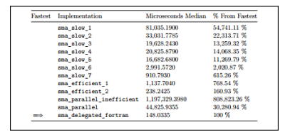
summary(performance)$meIn this case, our median time is of 148.0335 microseconds, making this the fastest implementation up to this point. Note that it’s barely over half of the time from the most efficient implementation we were able to come up with using only R. Take a look at the following table:
Boost R codes using a modern approach with C++
Now, we will show you how to use a more modern approach using C++. The aim of this section is to provide just enough information for you to start experimenting using C++ within R on your own. We will only look at a tiny piece of what can be done by interfacing R with C++ through the Rcpp package (which is installed by default in R), but it should be enough to get you started.
If you have never heard of C++, it’s a language used mostly when resource restrictions play an important role and performance optimization is of paramount importance. Some good resources to learn more about C++ are Meyer’s books on the topic, a popular one being Effective C++ (Addison-Wesley, 2005), and specifically for the Rcpp package, Eddelbuettel’s Seamless R and C++ integration with Rcpp by Springer, 2013, is great.
Before we continue, you need to ensure that you have a C++ compiler in your system. On Linux, you should be able to use gcc. On Mac, you should install Xcode from the application store. O n Windows, you should install Rtools. Once you test your compiler and know that it’s working, you should be able to follow this section. We’ll cover more on how to do this in Appendix, Required Packages.
C++ is more readable than Fortran code because it follows more syntax conventions we’re used to nowadays. However, just because the example we will use is readable, don’t think that C++ in general is an easy language to use; it’s not. It’s a very low-level language and using it correctly requires a good amount of knowledge. Having said that, let’s begin.
The #include line is used to bring variable and function definitions from R into this file when it’s compiled. Literally, the contents of the Rcpp.h file are pasted right where the include statement is. Files ending with the .h extensions are called header files, and they are used to provide some common definitions between a code’s user and its developers.
The using namespace Rcpp line allows you to use shorter names for your function. Instead of having to specify Rcpp::NumericVector, we can simply use NumericVector to define the type of the data object. Doing so in this example may not be too beneficial, but when you start developing for complex C++ code, it will really come in handy.
Next, you will notice the // [[Rcpp::export(sma_delegated_cpp)]] code. This is a tag that marks the function right below it so that R know that it should import it and make it available within R code. The argument sent to export() is the name of the function that will be accessible within R, and it does not necessarily have to match the name of the function in C++. In this case, sma_delegated_cpp() will be the function we call within R, and it will call the smaDelegated() function within C++:
#include
using namespace Rcpp;
// [[Rcpp::export(sma_delegated_cpp)]]
NumericVector smaDelegated(int period, NumericVector data) {
int position, n = data.size();
NumericVector result(n);
double sma;
for (int end = 0; end < n; end++) {
position = end;
sma = 0;
while(end - position < period && position >= 0) {
sma = sma + data[position];
position = position - 1;
}
if (end - position == period) {
sma = sma / period;
} else {
sma = NA_REAL;
}
result[end] = sma;
}
return result;
}
Next, we will explain the actual smaDelegated() function. Since you have a good idea of what it’s doing at this point, we won’t explain its logic, only the syntax that is not so obvious. The first thing to note is that the function name has a keyword before it, which is the type of the return value for the function. In this case, it’s NumericVector, which is provided in the Rcpp.h file. This is an object designed to interface vectors between R and C++. Other types of vector provided by Rcpp are IntegerVector, LogicalVector, and CharacterVector. You also have IntegerMatrix, NumericMatrix, LogicalMatrix, and CharacterMatrix available.
Next, you should note that the parameters received by the function also have types associated with them. Specifically, period is an integer (int), and data is NumericVector, just like the output of the function. In this case, we did not have to pass the output or length objects as we did with Fortran. Since functions in C++ do have output values, it also has an easy enough way of computing the length of objects.
The first line in the function declare a variables position and n, and assigns the length of the data to the latter one. You may use commas, as we do, to declare various objects of the same type one after another instead of splitting the declarations and assignments into its own lines. We also declare the vector result with length n; note that this notation is similar
to Fortran’s. Finally, instead of using the real keyword as we do in Fortran, we use the float or double keyword here to denote such numbers. Technically, there’s a difference regarding the precision allowed by such keywords, and they are not interchangeable, but we won’t worry about that here.
The rest of the function should be clear, except for maybe the sma = NA_REAL assignment. This NA_REAL object is also provided by Rcpp as a way to denote what should be sent to R as an NA. Everything else should result familiar.
Now that our function is ready, we save it in a file called sma-delegated-cpp.cpp and use R’s sourceCpp() function to bring compile it for us and bring it into R. The .cpp extension denotes contents written in the C++ language. Keep in mind that functions brought into R from C++ files cannot be saved in a .Rdata file for a later session. The nature of C++ is to be very dependent on the hardware under which it’s compiled, and doing so will probably produce various errors for you. Every time you want to use a C++ function, you should compile it and load it with the sourceCpp() function at the moment of usage.
library(Rcpp)

sourceCpp("./sma-delegated-cpp.cpp")

sma_delegated_cpp <- function(period, symbol, data) {

data <- as.numeric(data[which(data$symbol == symbol), "price_usd"])

return(sma_cpp(period, data))

}
If everything worked fine, our function should be usable within R, so we benchmark and test for correctness. I promise this is the last one:
performance <- microbenchmark(

sma_13 <- sma_delegated_cpp(period, symboo, data),

unit = "us"

)

all(sma_1$sma - sma_13 <= 0.001, na.rm = TRUE)

#> TRUE

summary(performance)$median

#> [1] 80.6415
This time, our median time was 80.6415 microseconds, which is three orders of magnitude faster than our first implementation. Think about it this way: if you provide an input for sma_delegated_cpp() so that it took around one hour for it to execute, sma_slow_1() would take around 1,000 hours, which is roughly 41 days. Isn’t that a surprising difference? When you are in situations that take that much execution time, it’s definitely worth it to try and make your implementations as optimized as possible.
You may use the cppFunction() function to write your C++ code directly inside an .R file, but you should not do so. Keep that just for testing small pieces of code. Separating your C++ implementation into its own files allows you to use the power of your editor of choice (or IDE) to guide you through the development as well as perform deeper syntax checks for you.
You read an excerpt from R Programming By Example authored by Omar Trejo Navarro. This book provides step-by-step guide to build simple-to-advanced applications through examples in R using modern tools.
Read Next
Getting Inside a C++ Multithreaded Application
Understanding the Dependencies of a C++ Application


