


In this article by Michael Heydt, author of the book Learning Pandas – Second Edition, we will cover how to install pandas and start using its basic functionality. The content is provided as IPython and Jupyter notebooks, and hence we will also take a quick look at using both of those tools.
We will utilize the Anaconda Scientific Python distribution from Continuum. Anaconda is a popular Python distribution with both free and paid components. Anaconda provides cross-platform support—including Windows, Mac, and Linux. The base distribution of Anaconda installs pandas, IPython and Jupyter notebooks, thereby making it almost trivial to get started.
(For more resources related to this topic, see here.)
IPython and Jupyter Notebook
So far we have executed Python from the command line / terminal. This is the default Read-Eval-Print-Loop (REPL)that comes with Python. Let’s take a brief look at both.
IPython
IPython is an alternate shell for interactively working with Python. It provides several enhancements to the default REPL provided by Python.
If you want to learn about IPython in more detail check out the documentation at https://ipython.org/ipython-doc/3/interactive/tutorial.html
To start IPython, simply execute the ipython command from the command line/terminal. When started you will see something like the following:
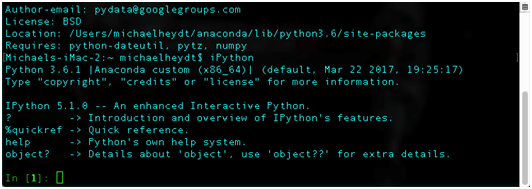
The input prompt which shows In [1]:. Each time you enter a statement in the IPythonREPL the number in the prompt will increase.
Likewise, output from any particular entry you make will be prefaced with Out [x]:where x matches the number of the corresponding In [x]:.The following demonstrates:
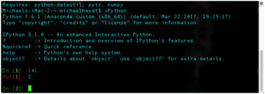
This numbering of in and out statements will be important to the examples as all examples will be prefaced with In [x]:and Out [x]: so that you can follow along.
Note that these numberings are purely sequential. If you are following through the code in the text and occur errors in input or enter additional statements, the numbering may get out of sequence (they can be reset by exiting and restarting IPython). Please use them purely as reference.
Jupyter Notebook
Jupyter Notebook is the evolution of IPython notebook. It is an open-source web application that allows you to create and share documents that contain live code, equations, visualizations, and markdown.
The original IPython notebook was constrained to Python as the only language. Jupyter Notebook has evolved to allow many programming languages to be used including Python, R, Julia, Scala, and F#.
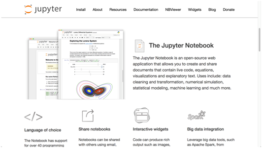
If you want to take a deeper look at Jupyter Notebook head to the following URL http://jupyter.org/: where you will be presented with a page similar to the following:
Jupyter Notebookcan be downloaded and used independently of Python. Anaconda does installs it by default. To start a Jupyter Notebookissue the following command at the command line/Terminal:
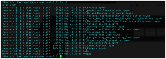
$ jupyter notebookTo demonstrate, let’s look at how to run the example code that comes with the text. Download the code from the Packt website and and unzip the file to a directory of your choosing. In the directory, you will see the following contents:
Now issue the jupyter notebook command. You should see something similar to the following:
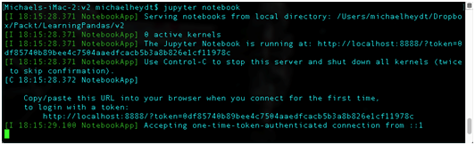
A browser page will open displaying the Jupyter Notebook homepage which is http://localhost:8888/tree. This will open a web browser window showing this page, which will be a directory listing:
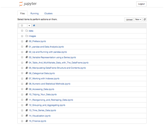
Clicking on a .ipynb link opens a notebook page like the following:
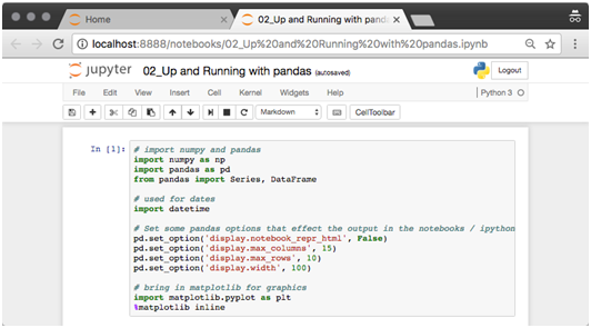
The notebook that is displayed is HTML that was generated by Jupyter and IPython. It consists of a number of cells that can be one of 4 types: code, markdown, raw nbconvert or heading.
Jupyter runs an IPython kernel for each notebook. Cells that contain Python code are executed within that kernel and the results added to the notebook as HTML.
Double-clicking on any of the cells will make the cell editable. When done editing the contents of a cell, press shift-return, at which point Jupyter/IPython will evaluate the contents and display the results.
If you wan to learn more about the notebook format that underlies the pages, see https://ipython.org/ipython-doc/3/notebook/nbformat.html.
The toolbar at the top of a notebook gives you a number of abilities to manipulate the notebook. These include adding, removing, and moving cells up and down in the notebook. Also available are commands to run cells, rerun cells, and restart the underlying IPython kernel.
To create a new notebook, go to File > New Notebook > Python 3 menu item.
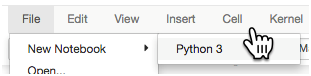
A new notebook page will be created in a new browser tab. Its name will be Untitled:
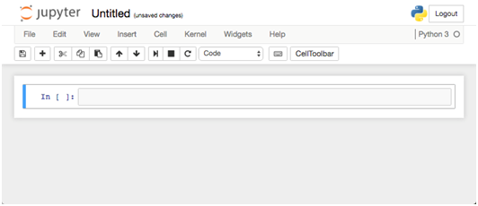
The notebook consists of a single code cell that is ready to have Python entered. EnterIPython1+1 in the cell and press Shift + Enter to execute.
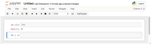
The cell has been executed and the result shown as Out [2]:. Jupyter also opened a new cellfor you to enter more code or markdown.
Jupyter Notebook automatically saves your changes every minute, but it’s still a good thing to save manually every once and a while.
One final point before we look at a little bit of pandas. Code in the text will be in the format of command -line IPython. As an example, the cell we just created in our notebook will be shown as follows:
In [1]: 1+1
Out [1]: 2
Introducing the pandas Series and DataFrame
Let’s jump into using some pandas with a brief introduction to pandas two main data structures, the Series and the DataFrame. We will examine the following:
- Importing pandas into your application
- Creating and manipulating a pandas Series
- Creating and manipulating a pandas DataFrame
- Loading data from a file into a DataFrame
The pandas Series
The pandas Series is the base data structure of pandas. A Series is similar to a NumPy array, but it differs by having an index which allows for much richer lookup of items instead of just a zero-based array index value.
The following creates a Series from a Python list.:
In  [2]: # create a four item Series
s = Series([1, 2, 3, 4])
         s

Out [2]:0    1
1    2
2    3
3    4
dtype: int64
The output consists of two columns of information. The first is the index and the second is the data in the Series. Each row of the output represents the index label (in the first column) and then the value associated with that label.
Because this Series was created without specifying an index (something we will do next), pandas automatically creates an integer index with labels starting at 0 and increasing by one for each data item.
The values of a Series object can then be accessed through the using the [] operator, paspassing the label for the value you require. The following gets the value for the label 1:
In  [3]:s[1]
Out [3]: 2
This looks very much like normal array access in many programming languages. But as we will see, the index does not have to start at 0, nor increment by one, and can be many other data types than just an integer. This ability to associate flexible indexes in this manner is one of the great superpowers of pandas.
Multiple items can be retrieved by specifying their labels in a python list. The following retrieves the values at labels 1 and 3:
In  [4]: # return a Series with the row with labels 1 and 3
s[[1, 3]]
Out [4]: 1    2
3    4
dtype: int64
A Series object can be created with a user-defined index by using the index parameter and specifying the index labels. The following creates a Series with the same valuesbut with an index consisting of string values:
In  [5]:# create a series using an explicit index
s = pd.Series([1, 2, 3, 4],
index = ['a', 'b', 'c', 'd'])
s
Out [5}:a    1
b    2
c    3
d    4
dtype: int64
Data in the Series object can now be accessed by those alphanumeric index labels. The following retrieves the values at index labels ‘a’ and ‘d’:
In [6]:# look up items the series having index 'a' and 'd'
s[['a', 'd']]
Out [6]:a    1
d    4
dtype: int64
It is still possible to refer to the elements of this Series object by their numerical 0-based position. :
In [7]:# passing a list of integers to a Series that has
# non-integer index labels will look up based upon
# 0-based index like an array
s[[1, 2]]
Out [7]:b    2
c    3
dtype: int64
We can examine the index of a Series using the .index property:
In [8]:# get only the index of the Series
s.index

Out [8]: Index(['a', 'b', 'c', 'd'], dtype='object')
The index is itself actually a pandas objectand this output shows us the values of the index and the data type used for the index. In this case note that the type of the data in the index (referred to as the dtype) is object and not string.
A common usage of a Series in pandas is to represent a time-series that associates date/time index labels withvalues. The following demonstrates by creating a date range can using the pandas function pd.date_range():
In  [9]:# create a Series who's index is a series of dates
# between the two specified dates (inclusive)
dates = pd.date_range('2016-04-01', '2016-04-06')
dates

Out [9]:DatetimeIndex(['2016-04-01', '2016-04-02', '2016-
04-03', '2016-04-04', '2016-04-05', '2016-04-06'],
dtype='datetime64[ns]', freq='D')
This has created a special index in pandas referred to as a DatetimeIndex which is a specialized type of pandas index that is optimized to index data with dates and times.
Now let’s create a Series using this index. The data values represent high-temperatures on those specific days:
In [10]:# create a Series with values (representing
temperatures)
# for each date in the index
temps1 = Series([80, 82, 85, 90, 83, 87],
     index = dates)
temps1

Out [10]:2016-04-01    80
2016-04-02    82
2016-04-03    85
2016-04-04    90
2016-04-05    83
2016-04-06    87
Freq: D, dtype: int64
This type of Series with a DateTimeIndexis referred to as a time-series.
We can look up a temperature on a specific data by using the date as a string:
In [11]:temps1['2016-04-04']
Out [11]:90
Two Series objects can be applied to each other with an arithmetic operation. The following code creates a second Series and calculates the difference in temperature between the two:
In  [12]:# create a second series of values using the same index
temps2 = Series([70, 75, 69, 83, 79, 77],
      index = dates)
# the following aligns the two by their index values
# and calculates the difference at those matching labels
temp_diffs = temps1 - temps2
temp_diffs

Out [12]:2016-04-01    10
2016-04-02     7
2016-04-03    16
2016-04-04     7
2016-04-05     4
2016-04-06    10
Freq: D, dtype: int64
The result of an arithmetic operation (+, -, /, *, …) on two Series objects that are non-scalar values returns another Series object.
Since the index is not integerwe can also then look up values by 0-based value:
In [13]:# and also possible by integer position as if the
# series was an array
temp_diffs[2]
Out [13]: 16
Finally, pandas provides many descriptive statistical methods. As an example, the following returns the mean of the temperature differences:
In [14]: # calculate the mean of the values in the Serie
temp_diffs
Out [14]: 9.0
The pandas DataFrame
A pandas Series can only have a single value associated with each index label. To have multiple values per index label we can use a DataFrame. A DataFrame represents one or more Series objects aligned by index label. Each Series will be a column in the DataFrame, and each column can have an associated name.—
In a way, a DataFrame is analogous to a relational database table in that it contains one or more columns of data of heterogeneous types (but a single type for all items in each respective column).
The following creates a DataFrame object with two columns and uses the temperature Series objects:
In [15]:# create a DataFrame from the two series objects temp1
          # and temp2 and give them column names
temps_df = DataFrame(
{'Missoula': temps1,
'Philadelphia': temps2})
temps_df
Out [15]:             Missoula  Philadelphia
          2016-04-01        80            70
          2016-04-02        82            75
          2016-04-03        85            69
          2016-04-04        90            83
          2016-04-05        83            79
          2016-04-06        87            77
The resulting DataFrame has two columns named Missoula and Philadelphia. These columns are new Series objects contained within the DataFrame with the values copied from the original Series objects.
Columns in a DataFrame object can be accessed using an array indexer [] with the name of the column or a list of column names. The following code retrieves the Missoula column:
In [16]:# get the column with the name Missoula
temps_df['Missoula']
Out [16]:2016-04-01    80
         2016-04-02    82
         2016-04-03    85
         2016-04-04    90
         2016-04-05    83
         2016-04-06    87
         Freq: D, Name: Missoula, dtype: int64
And the following code retrieves the Philadelphia column:
In  [17]:# likewise we can get just the Philadelphia column
temps_df['Philadelphia']
Out [17]:2016-04-01    70
         2016-04-02    75
         2016-04-03    69
         2016-04-04    83
         2016-04-05    79
         2016-04-06    77
         Freq: D, Name: Philadelphia, dtype: int64
A Python list of column names can also be used to return multiple columns.:
In [18]:# return both columns in a different order
temps_df[['Philadelphia', 'Missoula']]
Out [18]:             Philadelphia  Missoula
         2016-04-01            70        80
         2016-04-02            75        82
         2016-04-03            69        85
         2016-04-04            83        90
         2016-04-05            79        83
         2016-04-06            77        87
There is a subtle difference in a DataFrame object as compared to a Series object. Passing a list to the [] operator of DataFrame retrieves the specified columns whereas aSerieswould return rows.
If the name of a column does not have spaces it can be accessed using property-style:
In [19]:# retrieve the Missoula column through property syntax
temps_df.Missoula
Out [19]:2016-04-01    80
         2016-04-02    82
         2016-04-03    85
         2016-04-04    90
         2016-04-05    83
         2016-04-06    87
         Freq: D, Name: Missoula, dtype: int64
Arithmetic operations between columns within a DataFrame are identical in operation to those on multiple Series. To demonstrate, the following code calculates the difference between temperatures using property notation:
In  [20]:# calculate the temperature difference between the two
          #cities
temps_df.Missoula - temps_df.Philadelphia
Out [20]:2016-04-01    10
         2016-04-02     7
         2016-04-03    16
         2016-04-04     7
         2016-04-05     4
         2016-04-06    10
         Freq: D, dtype: int64
A new column can be added to DataFrame simply by assigning another Series to a column using the array indexer [] notation. The following adds a new column in the DataFrame with the temperature differences:
In  [21]:# add a column to temp_df which contains the difference
          # in temps
temps_df['Difference'] = temp_diffs
temps_df
Out [21]:            Missoula  Philadelphia  Difference
        2016-04-01        80            70          10
        2016-04-02        82            75           7
        2016-04-03        85            69          16
        2016-04-04        90            83           7
        2016-04-05        83            79           4
        2016-04-06        87            77          10
The names of the columns in a DataFrame are accessible via the.columns property. :
In [22]:# get the columns, which is also an Index object
temps_df.columns

Out [22]:Index(['Missoula', 'Philadelphia', 'Difference'],
                dtype='object')
The DataFrame (and Series) objects can be sliced to retrieve specific rows. The following slices the second through fourth rows of temperature difference values:
In [23]:# slice the temp differences column for the rows at
# location 1 through 4 (as though it is an array)
temps_df.Difference[1:4]
Out [23]: 2016-04-02     7
2016-04-03    16
2016-04-04     7
Freq: D, Name: Difference, dtype: int64
Entire rows from a DataFrame can be retrieved using the .loc and .iloc properties. .loc ensures that the lookup is by index label, where .iloc uses the 0-based position. –
The following retrieves the second row of the DataFrame.
In[24]:# get the row at array position 1
temps_df.iloc[1]
Out [24]:Missoula        82
Philadelphia    75
Difference       7
Name: 2016-04-02 00:00:00, dtype: int64
Notice that this result has converted the row into a Series with the column names of the DataFrame pivoted into the index labels of the resulting Series.The following shows the resulting index of the result.
In [25]:# the names of the columns have become the index
# they have been 'pivoted'
temps_df.iloc[1].index

Out [25]:Index(['Missoula', 'Philadelphia', 'Difference'],
dtype='object')
Rows can be explicitly accessed via index label using the .loc property. The following code retrieves a row by the index label:
In  [26]:# retrieve row by index label using .loc
temps_df.loc['2016-04-05']
Out [26]:Missoula        83
Philadelphia    79
Difference       4
Name: 2016-04-05 00:00:00, dtype: int64
Specific rows in a DataFrame object can be selected using a list of integer positions. The following selects the values from the Differencecolumn in rows at integer-locations 1, 3, and 5:
In  [27]:# get the values in the Differences column in rows 1, 3
          # and 5using 0-based location
temps_df.iloc[[1, 3, 5]].Difference

Out [27]:2016-04-02     7
2016-04-04     7
2016-04-06    10
Freq: 2D, Name: Difference, dtype: int64
Rows of a DataFrame can be selected based upon a logical expression that is applied to the data in each row. The following shows values in the Missoulacolumn that are greater than 82 degrees:
In  [28]:# which values in the Missoula column are > 82?
temps_df.Missoula > 82

Out [28]:2016-04-01    False
2016-04-02    False
2016-04-03     True
2016-04-04     True
2016-04-05     True
2016-04-06     True
Freq: D, Name: Missoula, dtype: bool
The results from an expression can then be applied to the[] operator of a DataFrame (and a Series) which results in only the rows where the expression evaluated to Truebeing returned:
In  [29]:# return the rows where the temps for Missoula > 82
temps_df[temps_df.Missoula > 82]

Out [29]:   Missoula  Philadelphia  Difference
2016-04-03        85            69          16
2016-04-04        90            83           7
2016-04-05        83            79           4
2016-04-06        87            77          10
This technique is referred to as boolean election in pandas terminologyand will form the basis of selecting rows based upon values in specific columns (like a query in —SQL using a WHERE clause – but as we will see also being much more powerful).
Visualization
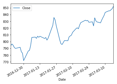
We will dive into visualization in quite some depth in Chapter 14, Visualization, but prior to then we will occasionally perform a quick visualization of data in pandas. Creating a visualization of data is quite simple with pandas. All that needs to be done is to call the .plot() method. The following demonstrates by plotting the Close value of the stock data.
In  [40]:
df[['Close']].plot();
Summary
In this article, took an introductory look at the pandas Series and DataFrame objects, demonstrating some of the fundamental capabilities. This exposition showed you how to perform a few basic operations that you can use to get up and running with pandas prior to diving in and learning all the details.
Resources for Article:
Further resources on this subject:
- Using indexes to manipulate pandas objects [article]
- Predicting Sports Winners with Decision Trees and pandas [article]
- The pandas Data Structures [article]