


Understanding the basic building blocks of a neural network, such as tensors, tensor operations, and gradient descents, is important for building complex neural networks. In this article, we will build our first Hello world program in PyTorch.
This tutorial is taken from the book Deep Learning with PyTorch. In this
book, you will build neural network models in text, vision and advanced analytics using PyTorch.
Let’s assume that we work for one of the largest online companies, Wondermovies, which serves videos on demand. Our training dataset contains a feature that represents the average hours spent by users watching movies on the platform and we would like to predict how much time each user would spend on the platform in the coming week. It’s just an imaginary use case, don’t think too much about it. Some of the high-level activities for building such a solution are as follows:
- Data preparation: The get_data function prepares the tensors (arrays) containing input and output data
- Creating learnable parameters: The get_weights function provides us with tensors containing random values that we will optimize to solve our problem
- Network model: The simple_network function produces the output for the input data, applying a linear rule, multiplying weights with input data, and adding the bias term (y = Wx+b)
- Loss: The loss_fn function provides information about how good the model is
- Optimizer: The optimize function helps us in adjusting random weights created initially to help the model calculate target values more accurately
Let’s consider following linear regression equation for our neural network:

Let’s write our first neural network in PyTorch:
x,y = get_data() # x - represents training data,y - represents target variables
w,b = get_weights() # w,b – Learnable parameters
for i in range(500):
y_pred = simple_network(x) # function which computes wx + b
loss = loss_fn(y,y_pred) # calculates sum of the squared differences of y and y_pred
if i % 50 == 0:
print(loss)
optimize(learning_rate) # Adjust w,b to minimize the loss
Data preparation
PyTorch provides two kinds of data abstractions called tensors and variables. Tensors are similar to numpy arrays and they can also be used on GPUs, which provide increased performance. They provide easy methods of switching between GPUs and CPUs. For certain operations, we can notice a boost in performance and machine learning algorithms can understand different forms of data, only when represented as tensors of numbers. Tensors are like Python arrays and can change in size.
Scalar (0-D tensors)
A tensor containing only one element is called a scalar. It will generally be of type FloatTensor or LongTensor. At the time of writing, PyTorch does not have a special tensor with zero dimensions. So, we use a one-dimension tensor with one element, as follows:
x = torch.rand(10)
x.size()
Output – torch.Size([10])
Vectors (1-D tensors)
A vector is simply an array of elements. For example, we can use a vector to store the average temperature for the last week:
temp = torch.FloatTensor([23,24,24.5,26,27.2,23.0])
temp.size()
Output – torch.Size([6])
Matrix (2-D tensors)
Most of the structured data is represented in the form of tables or matrices. We will use a dataset called Boston House Prices, which is readily available in the Python scikit-learn machine learning library. The dataset is a numpy array consisting of 506 samples or rows and 13 features representing each sample. Torch provides a utility function called from_numpy(), which converts a numpy array into a torch tensor. The shape of the resulting tensor is 506 rows x 13 columns:
boston_tensor = torch.from_numpy(boston.data)
boston_tensor.size()
Output: torch.Size([506, 13])
boston_tensor[:2]
Output:
Columns 0 to 7
0.0063 18.0000 2.3100 0.0000 0.5380 6.5750 65.2000 4.0900
0.0273 0.0000 7.0700 0.0000 0.4690 6.4210 78.9000 4.9671
Columns 8 to 12
1.0000 296.0000 15.3000 396.9000 4.9800
2.0000 242.0000 17.8000 396.9000 9.1400
[torch.DoubleTensor of size 2×13]
3-D tensors
When we add multiple matrices together, we get a 3-D tensor. 3-D tensors are used to represent data-like images. Images can be represented as numbers in a matrix, which are stacked together. An example of an image shape is 224, 224, 3, where the first index represents height, the second represents width, and the third represents a channel (RGB). Let’s see how a computer sees a panda, using the next code snippet:
from PIL import Image
# Read a panda image from disk using a library called PIL and convert it to numpy array
panda = np.array(Image.open('panda.jpg').resize((224,224)))
panda_tensor = torch.from_numpy(panda)
panda_tensor.size()
Output - torch.Size([224, 224, 3])
#Display panda
plt.imshow(panda)
Since displaying the tensor of size 224, 224, 3 would occupy a couple of pages in the book, we will display the image and learn to slice the image into smaller tensors to visualize it:

Slicing tensors
A common thing to do with a tensor is to slice a portion of it. A simple example could be choosing the first five elements of a one-dimensional tensor; let’s call the tensor sales. We use a simple notation, sales[:slice_index] where slice_index represents the index where you want to slice the tensor:
sales = torch.FloatTensor([1000.0,323.2,333.4,444.5,1000.0,323.2,333.4,444.5])
sales[:5]
1000.0000
323.2000
333.4000
444.5000
1000.0000
[torch.FloatTensor of size 5]

sales[:-5]
1000.0000
323.2000
333.4000
[torch.FloatTensor of size 3]
Let’s do more interesting things with our panda image, such as see what the panda image looks like when only one channel is chosen and see how to select the face of the panda.
Here, we select only one channel from the panda image:
plt.imshow(panda_tensor[:,:,0].numpy())
#0 represents the first channel of RGB
The output is as follows:

Now, let’s crop the image. Say we want to build a face detector for pandas and we need just the face of a panda for that. We crop the tensor image such that it contains only the panda’s face:
plt.imshow(panda_tensor[25:175,60:130,0].numpy())
The output is as follows:

Another common example would be where you need to pick a specific element of a tensor:
#torch.eye(shape) produces an diagonal matrix with 1 as it diagonal #elements.
sales = torch.eye(3,3)
sales[0,1]
Output- 0.00.0
4-D tensors
One common example for four-dimensional tensor types is a batch of images. Modern CPUs and GPUs are optimized to perform the same operations on multiple examples faster. So, they take a similar time to process one image or a batch of images. So, it is common to use a batch of examples rather than use a single image at a time. Choosing the batch size is not straightforward; it depends on several factors. One major restriction for using a bigger batch or the complete dataset is GPU memory limitations—16, 32, and 64 are commonly used batch sizes.
Let’s look at an example where we load a batch of cat images of size 64 x 224 x 224 x 3 where 64 represents the batch size or the number of images, 244 represents height and width, and 3 represents channels:
#Read cat images from disk
cats = glob(data_path+'*.jpg')
#Convert images into numpy arrays
cat_imgs = np.array([np.array(Image.open(cat).resize((224,224))) for cat in cats[:64]])
cat_imgs = cat_imgs.reshape(-1,224,224,3)
cat_tensors = torch.from_numpy(cat_imgs)
cat_tensors.size()
Output – torch.Size([64, 224, 224, 3])
Tensors on GPU
We have learned how to represent different forms of data in a tensor representation. Some of the common operations we perform once we have data in the form of tensors are addition, subtraction, multiplication, dot product, and matrix multiplication. All of these operations can be either performed on the CPU or the GPU. PyTorch provides a simple function called cuda() to copy a tensor on the CPU to the GPU. We will take a look at some of the operations and compare the performance between matrix multiplication operations on the CPU and GPU.
Tensor addition can be obtained by using the following code:
#Various ways you can perform tensor addition
a = torch.rand(2,2)
b = torch.rand(2,2)
c = a + b
d = torch.add(a,b)
#For in-place addition
a.add_(5)
#Multiplication of different tensors
a*b
a.mul(b)
#For in-place multiplication
a.mul_(b)
For tensor matrix multiplication, let’s compare the code performance on CPU and GPU. Any tensor can be moved to the GPU by calling the .cuda() function.
Multiplication on the GPU runs as follows:
a = torch.rand(10000,10000)
b = torch.rand(10000,10000)
a.matmul(b)
Time taken: 3.23 s
#Move the tensors to GPU
a = a.cuda()
b = b.cuda()
a.matmul(b)
Time taken: 11.2 µs
These fundamental operations of addition, subtraction, and matrix multiplication can be used to build complex operations, such as a Convolution Neural Network (CNN) and a recurrent neural network (RNN).
Variables
Deep learning algorithms are often represented as computation graphs. Here is a simple example of the variable computation graph that we built in our example:

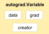
Each circle in the preceding computation graph represents a variable. A variable forms a thin wrapper around a tensor object, its gradients, and a reference to the function that created it. The following figure shows Variable class components:
The gradients refer to the rate of the change of the loss function with respect to various parameters (W, b). For example, if the gradient of a is 2, then any change in the value of a would modify the value of Y by two times. If that is not clear, do not worry—most of the deep learning frameworks take care of calculating gradients for us. In this part, we learn how to use these gradients to improve the performance of our model.
Apart from gradients, a variable also has a reference to the function that created it, which in turn refers to how each variable was created. For example, the variable a has information that it is generated as a result of the product between X and W.
Let’s look at an example where we create variables and check the gradients and the function reference:
x = Variable(torch.ones(2,2),requires_grad=True)
y = x.mean()
y.backward()

x.grad
Variable containing: 0.2500 0.2500 0.2500 0.2500 [torch.FloatTensor of size 2x2]

x.grad_fn
Output - None

x.data
1 1
1 1
[torch.FloatTensor of size 2x2]

y.grad_fn
<torch.autograd.function.MeanBackward at 0x7f6ee5cfc4f8>
In the preceding example, we called a backward operation on the variable to compute the gradients. By default, the gradients of the variables are none.
The grad_fn of the variable points to the function it created. If the variable is created by a user, like the variable x in our case, then the function reference is None. In the case of variable y, it refers to its function reference, MeanBackward.
The Data attribute accesses the tensor associated with the variable.
Creating data for our neural network
The get_data function in our first neural network code creates two variables, x and y, of sizes (17, 1) and (17). We will take a look at what happens inside the function:
def get_data():
    train_X = np.asarray([3.3,4.4,5.5,6.71,6.93,4.168,9.779,6.182,7.59,2.167,
                         7.042,10.791,5.313,7.997,5.654,9.27,3.1])
    train_Y = np.asarray([1.7,2.76,2.09,3.19,1.694,1.573,3.366,2.596,2.53,1.221,
                         2.827,3.465,1.65,2.904,2.42,2.94,1.3])
    dtype = torch.FloatTensor
    X = Variable(torch.from_numpy(train_X).type(dtype),requires_grad=False).view(17,1)
    y = Variable(torch.from_numpy(train_Y).type(dtype),requires_grad=False)
    return X,y
Creating learnable parameters
In our neural network example, we have two learnable parameters, w and b, and two fixed parameters, x and y. We have created variables x and y in our get_data function. Learnable parameters are created using random initialization and have the require_grad parameter set to True, unlike x and y, where it is set to False. Let’s take a look at our get_weights function:
def get_weights():
    w = Variable(torch.randn(1),requires_grad = True)
    b = Variable(torch.randn(1),requires_grad=True)
    return w,b
Most of the preceding code is self-explanatory; torch.randn creates a random value of any given shape.
Neural network model
Once we have defined the inputs and outputs of the model using PyTorch variables, we have to build a model which learns how to map the outputs from the inputs. In traditional programming, we build a function by hand coding different logic to map the inputs to the outputs. However, in deep learning and machine learning, we learn the function by showing it the inputs and the associated outputs. In our example, we implement a simple neural network which tries to map the inputs to outputs, assuming a linear relationship. The linear relationship can be represented as y = wx + b, where w and b are learnable parameters. Our network has to learn the values of w and b, so that wx + b will be closer to the actual y. Let’s visualize our training dataset and the model that our neural network has to learn:

The following figure represents a linear model fitted on input data points:

The dark-gray (blue) line in the image represents the model that our network learns.
Network implementation
As we have all the parameters (x, w, b, and y) required to implement the network, we perform a matrix multiplication between w and x. Then, sum the result with b. That will give our predicted y. The function is implemented as follows:
def simple_network(x):
    y_pred = torch.matmul(x,w)+b
    return y_pred
PyTorch also provides a higher-level abstraction in torch.nn called layers, which will take care of most of these underlying initialization and operations associated with most of the common techniques available in the neural network. We are using the lower-level operations to understand what happens inside these functions. The previous model can be represented as a torch.nn layer, as follows:
f = nn.Linear(17,1) # Much simpler.
Now that we have calculated the y values, we need to know how good our model is, which is done in the loss function.
Loss function
As we start with random values, our learnable parameters, w and b, will result in y_pred, which will not be anywhere close to the actual y. So, we need to define a function which tells the model how close its predictions are to the actual values. Since this is a regression problem, we use a loss function called the sum of squared error (SSE). We take the difference between the predicted y and the actual y and square it. SSE helps the model to understand how close the predicted values are to the actual values. The torch.nn library has different loss functions, such as MSELoss and cross-entropy loss. However, for this chapter, let’s implement the loss function ourselves:
def loss_fn(y,y_pred):
    loss = (y_pred-y).pow(2).sum()
    for param in [w,b]:
        if not param.grad is None: param.grad.data.zero_()
    loss.backward()
    return loss.data[0]
Apart from calculating the loss, we also call the backward operation, which calculates the gradients of our learnable parameters, w and b. As we will use the loss function more than once, we remove any previously calculated gradients by calling the grad.data.zero_() operation. The first time we call the backward function, the gradients are empty, so we zero the gradients only when they are not None.
Optimize the neural network
We started with random weights to predict our targets and calculate loss for our algorithm. We calculate the gradients by calling the backward function on the final loss variable. This entire process repeats for one epoch, that is, for the entire set of examples. In most of the real-world examples, we will do the optimization step per iteration, which is a small subset of the total set. Once the loss is calculated, we optimize the values with the calculated gradients so that the loss reduces, which is implemented in the following function:
def optimize(learning_rate):
    w.data -= learning_rate * w.grad.data
    b.data -= learning_rate * b.grad.data
The learning rate is a hyper-parameter, which allows us to adjust the values in the variables by a small amount of the gradients, where the gradients denote the direction in which each variable (w and b) needs to be adjusted.
Different optimizers, such as Adam, RmsProp, and SGD are already implemented for use in the torch.optim package.
The final network architecture is a model for learning to predict average hours spent by users on our Wondermovies platform.
Next, to learn PyTorch built-in modules for building network architectures, read our book Deep Learning with PyTorch.
Read Next
Can a production ready Pytorch 1.0 give TensorFlow a tough time?


